Project 2: Fun with Filters and Frequencies!

Overview

This project explores using filters to manipulate the frequencies in images to alter their depiction. In Part 1, we look at filters--namely the derivative and Gaussian filters. We note that the derivative filter is an edge detector, and that Gaussian filters are low pass filters. In Part 2, we alter the frequency spectra of images. We can create "sharpening" filters that complement the Gaussian filters this way. Additionally, we can create "hybrid images" that portray one image close up (high frequencies) and one image from afar (low frequencies). In Part 3, we perform multiresolution blending.

Part 1: Fun with Filters

1.1 Finite Difference Operator

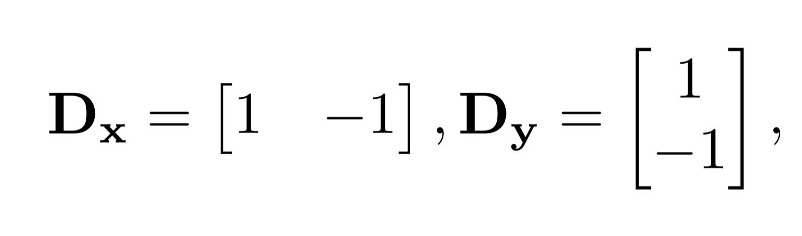
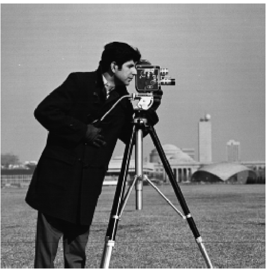
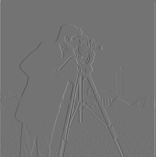
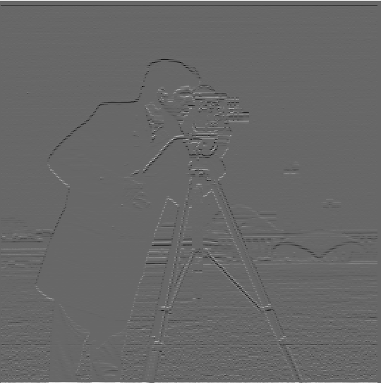
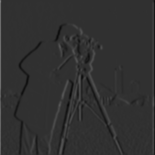
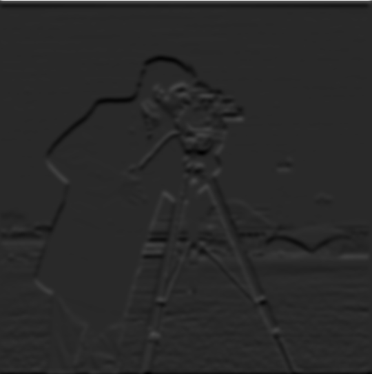
The finite difference operators shown above are filters that can show the derivative in the x and y directions. By convolving these operators with an image, you can see the partial derivative. Note that Dx shows vertical edges and Dy shows horizontal ones.

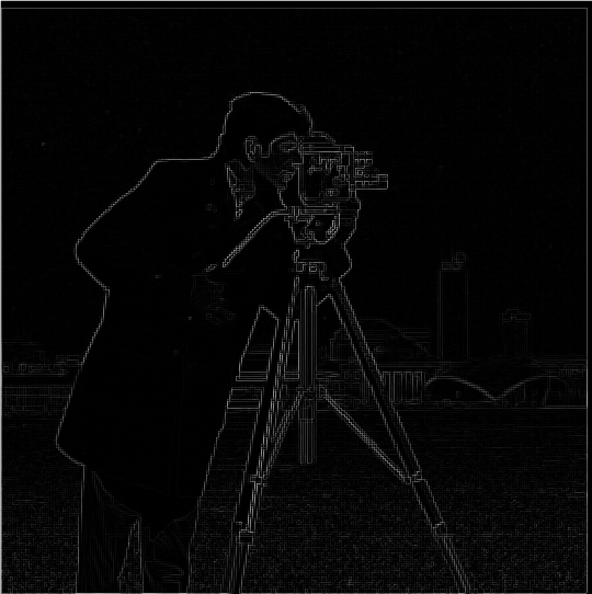
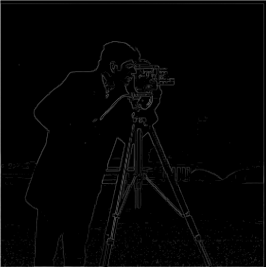
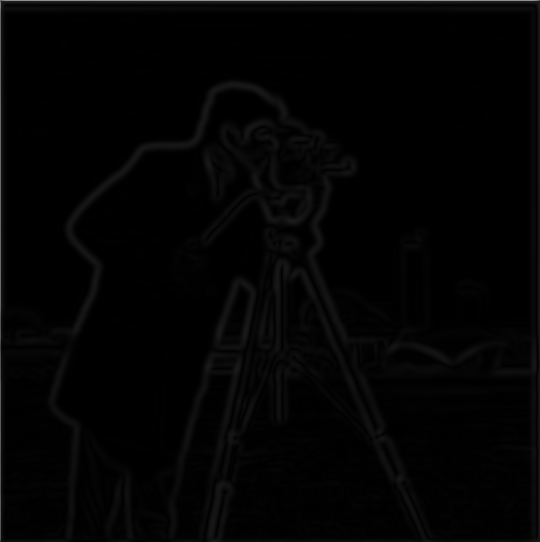
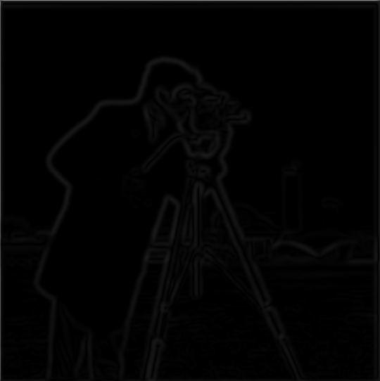
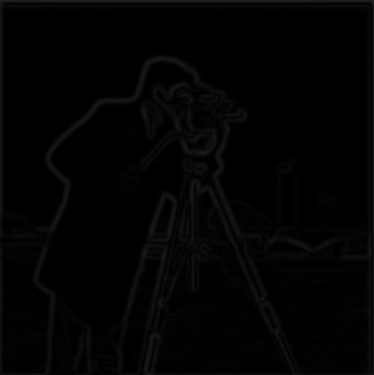
We can find a gradient magnitude image by taking the square root of the squares of the pixel values of Figure 2B and 2C (the norm). This is a measure of how strong the edge is in the image. However, you can note that there is some noise in the produced image. Therefore we can generate an edge image by suppressing any edges that have a magnitude less than some threshold. The gradient image and edge image for the cameraman.png are below. You'll note that there is less noise present in 3B in the area where there is originally grass.

1.2 Derivative of Gaussian (DoG) Filter

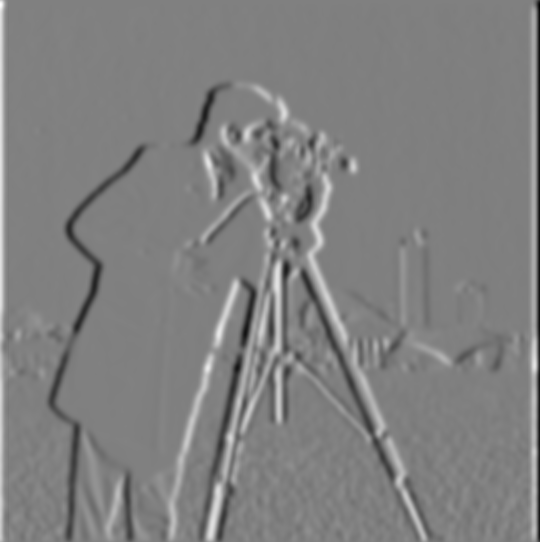
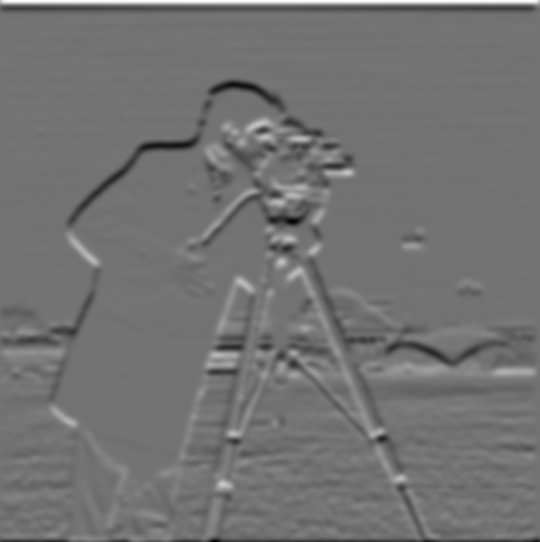
Because the images resulting from the difference operator were noisy, we can blur the image before taking the difference operator. This reduces the noise. To blur the image, we convolve the image with a Gaussian. This particular Gaussian is the outer product of the Gaussian with kernel size 15 and sigma of 3. The sigma indicates the spread of the Gaussian (how much the weights of the pixels are), and the kernel size dictates how many pixel values are considered in each blur step.

Below are the results of the Dx, Dy, gradient magnitude, and edge image functions. Note that the threshold for the edge image is basically 0. From the gradient magnitude image, you can see that blurring has already gotten ride of the noise. The overall image has much less noise and has a generally "softer" appearance. This is also why you must look more closely at the images to detect the edges; they are not as sharp and defined.

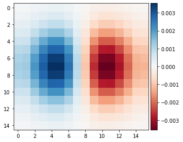
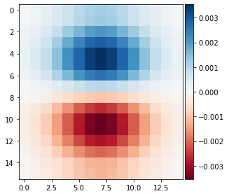
An important thing to note is that instead of creating a derivative filter and a Gaussian filter and convolving the image once with each, we can create a single filter for a single convolution. This single filter is a derivative of a Gaussian. We convolve the derivative filter with the Gaussian. As such we get the following filters.

Note that Figures 4D/4E and 5E are visually the same. This is because we have done the equivalent operations. One blurs then takes the derivatives. One takes the derivative of the blurs. Both combine the results at the end to generate an edge image.

Part 2: Fun with Frequencies

2.1 Image "Sharpening"

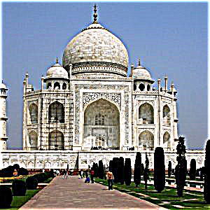
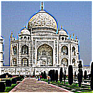
To artifically generate a "sharper" image, we can apply an unsharp mask filter to an existing image. An unsharp mask filter is the equivalent of subtracting a blurred version of the image (with only low frequencies) from the original image, leaving only the high frequencies. These high frequencies are what create this "sharpened" feel to the image. This is the equivalent to convolving using the above convolution. Note that the alphas are a parameter that dictates the extent of/severity of sharpness. Below are the results for varying alpha

While the results for alpha=1,2 seem acceptable and seem to enhance details (Figures 7B, 7C), we quickly see visually jarring artifacts for higher alphas. This is because the filter cannot provide any new information. It is simply exaggerating the information already in the image. For a truly "sharper" image, you would need a higher quality camera lens. This is more pronounced in the examples below. We present the original image, a blurred image (removing information), and then a sharpened version of the blurred image. It seems passable in Figure 8 (though again visually jarring), but the results are clearly inferior in Figure 9. You can tell by looking at the texture of the cat's fur. You cannot recover the original image; in the sharpened version, the cat's fur is has clearly exaggerated contrast. Examining the text closely will also expose some artifacts.

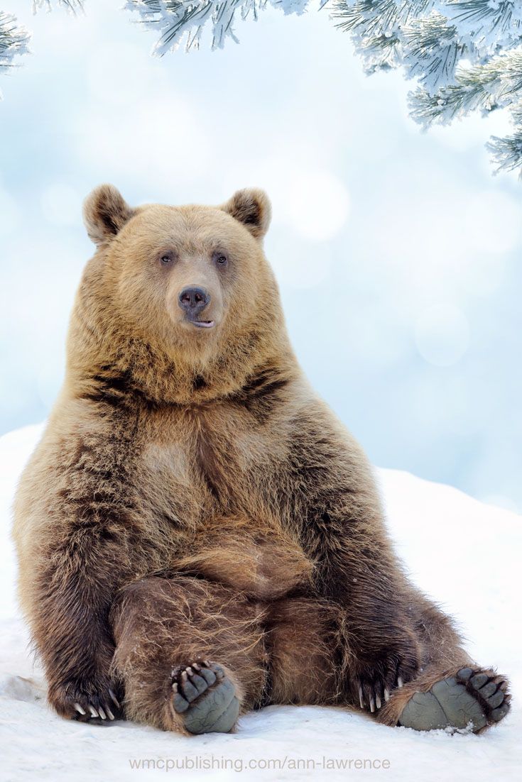
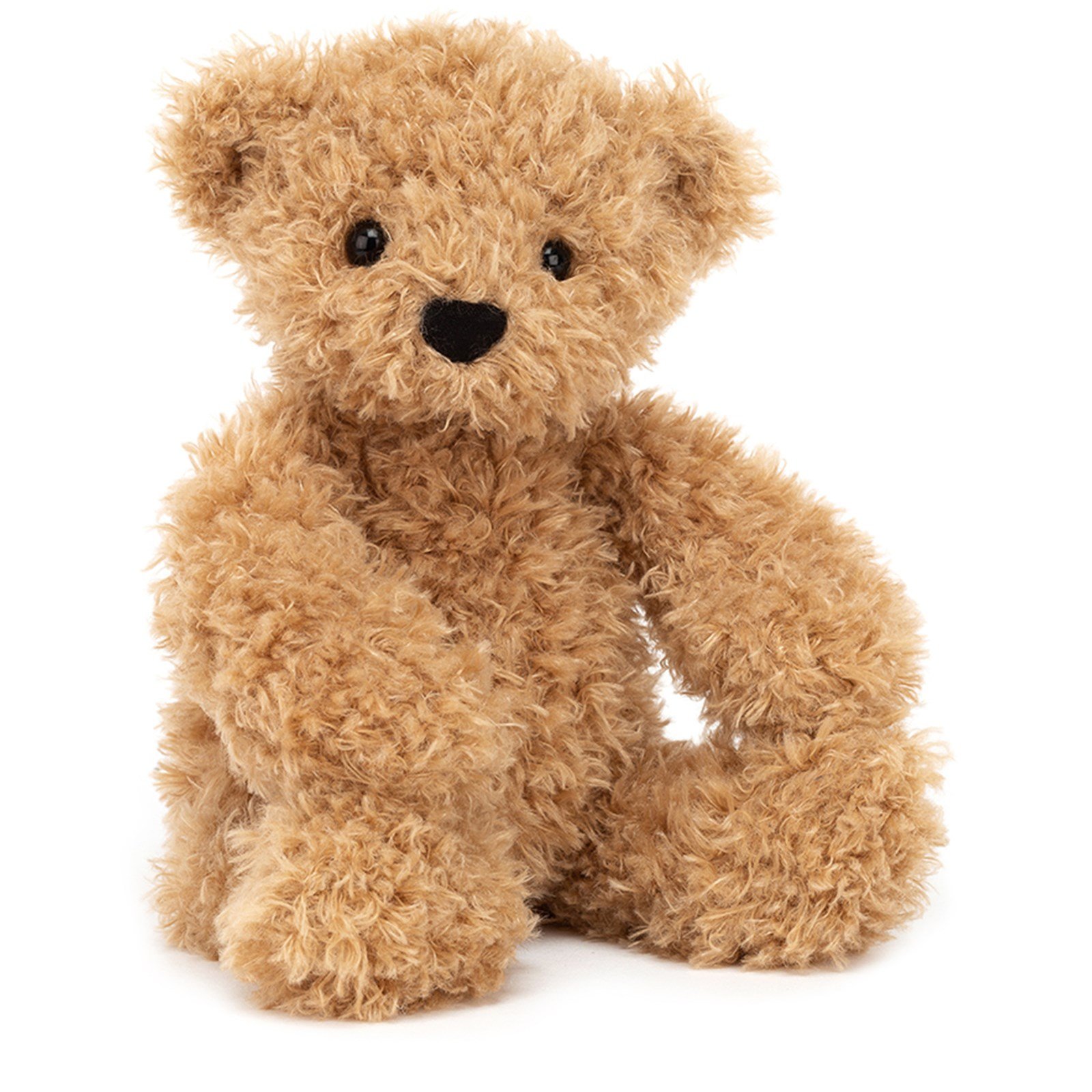
2.2: Hybrid Images

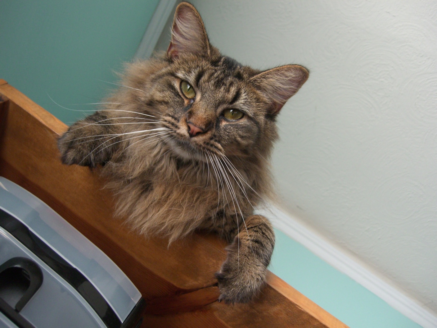
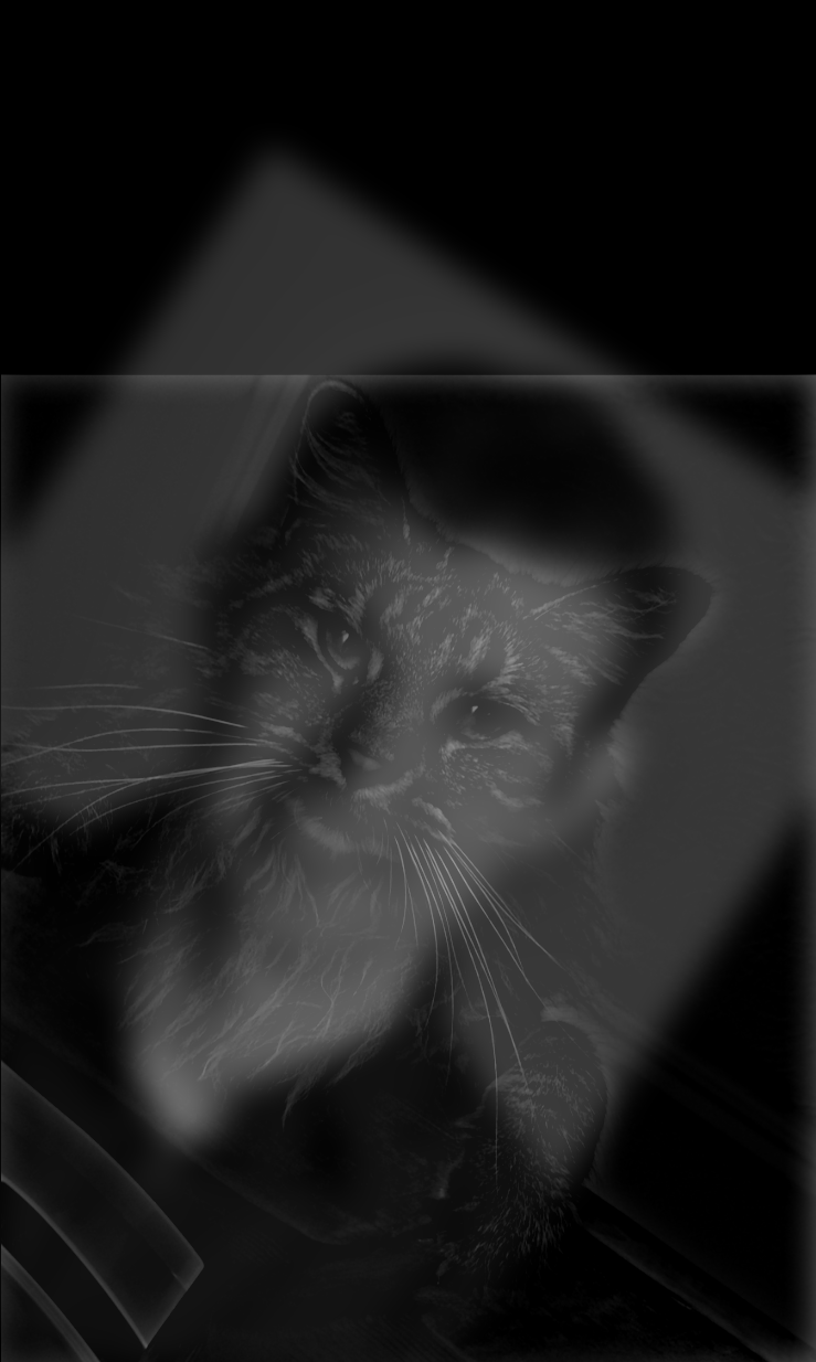
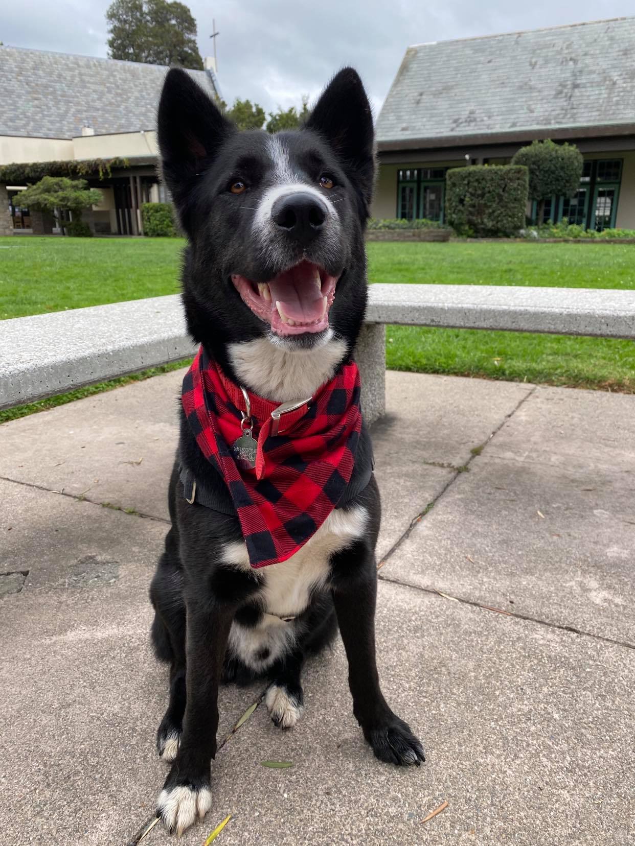
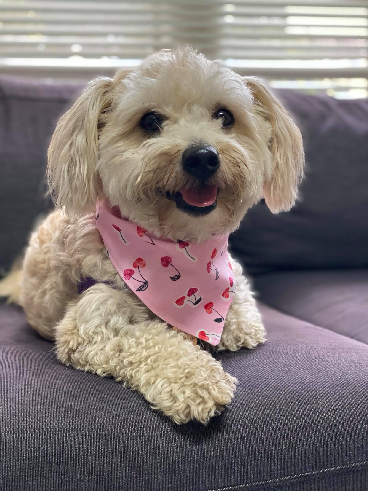
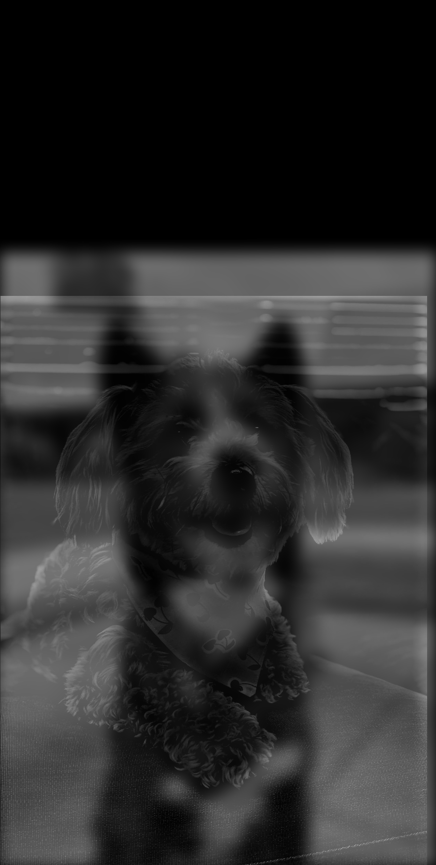
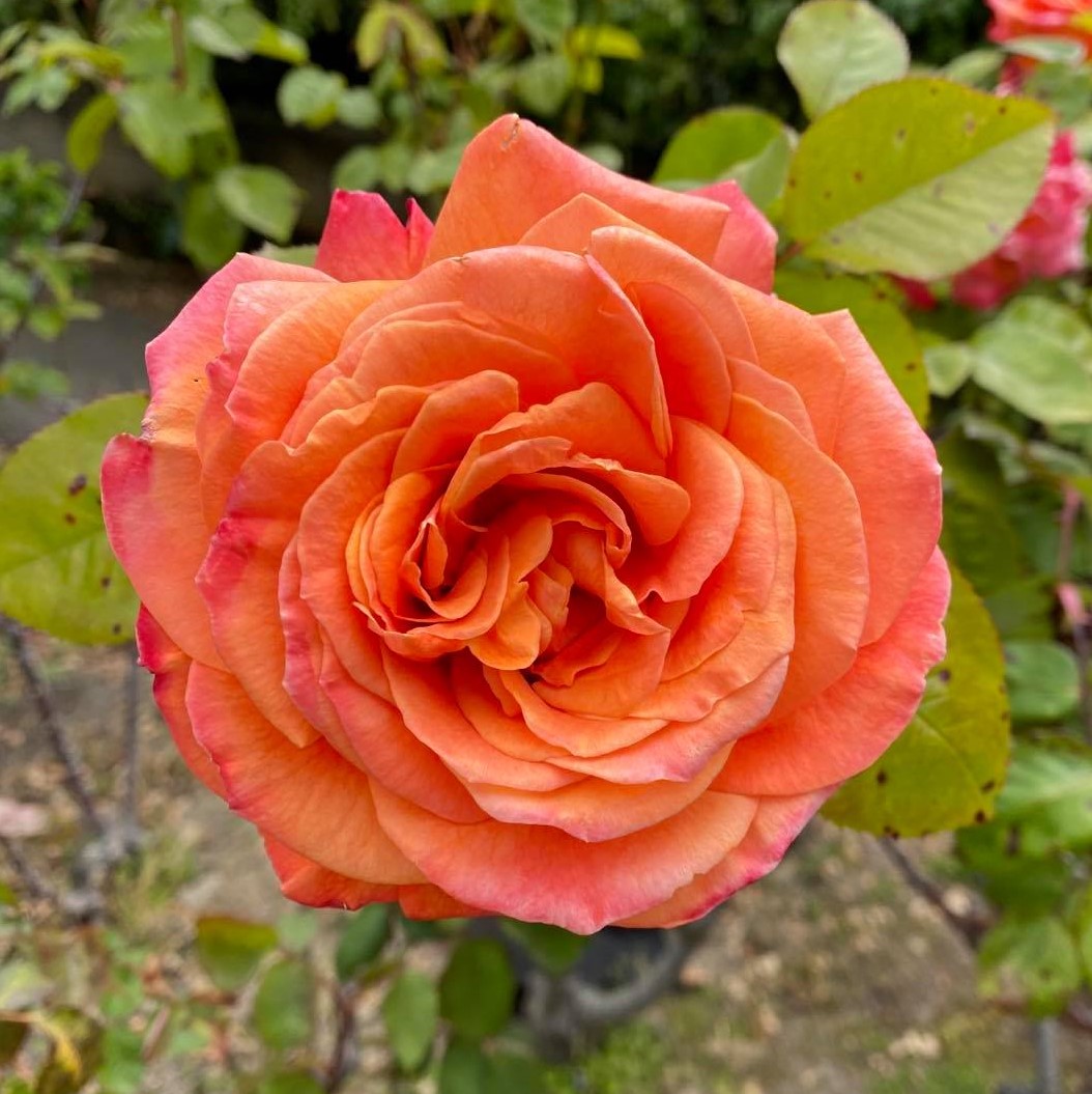
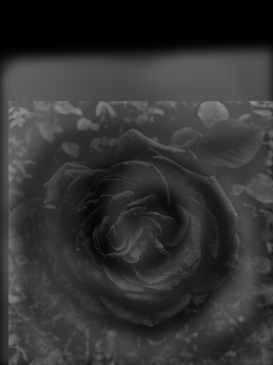
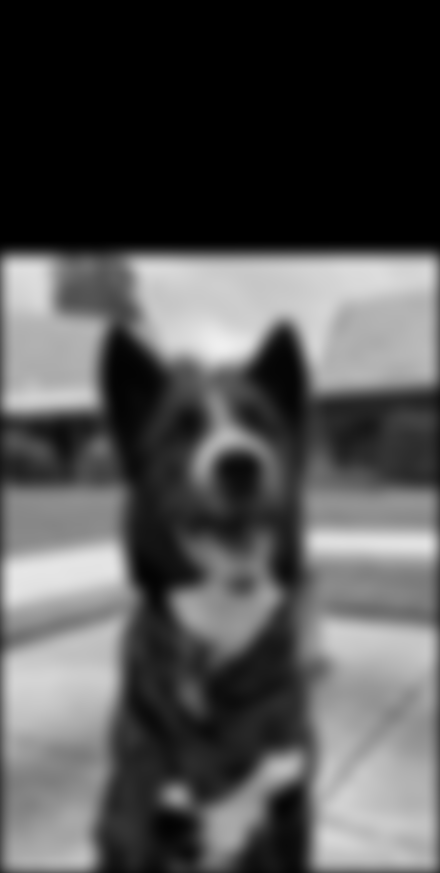
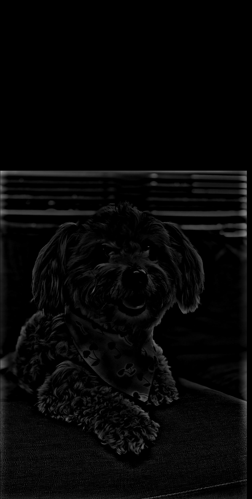
Humans perceive images differently based on the distance from the image. Up close, an image's high frequencies dominate the person's perception of the image. From far away, an image's low frequencies dominate the perception. We can take advantage of this fact and generate hybrid images. We pluck out the high frequencies of one image, the low frequencies of another, and then stack the filtered images on top of each other. This gives us one picture that has two images hidden in it, each accessible at different distances from the picture.

For the low pass filter (to retain low frequencies), we use a standard Gaussian of kernel size 60. The sigma varies on the image, as it dictates the cutoff frequency of the filter. For the high pass filter, we use a Laplacian of a Gaussian, or the impulse minus the Gaussian. This Gaussian also has a kernel size 60 and a varying sigma.

It is important to note that the images must be aligned in order for the result to be interesting. It is difficult to find images that align well. Additionally, we want to include the more textured image at the higher frequencies and the less textured image at the lower frequencies. Below are some interesting results.

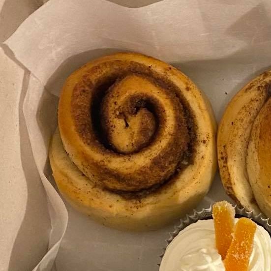
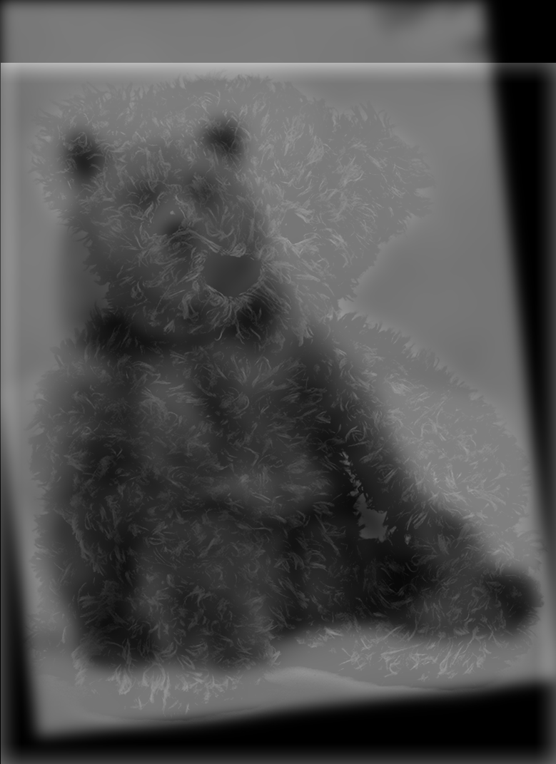
Of the above results, Figure 13 can be considered a failure. The alignment does not work particularly well, and additionally, you lose quite a bit of context from losing different frequencies. The blurred bear is not particularly evident from far away, probably also from context (how many real bears sit like this?). Similarly, it is hard in Figure 12 to decipher that it is a blurred cinnamon roll as opposed to a generic spiral. We lose quite a bit of information doing this.

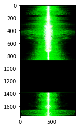
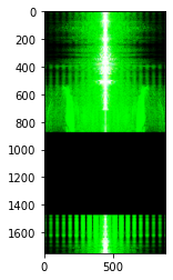
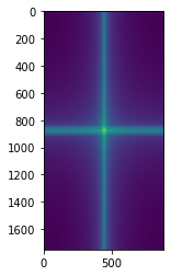
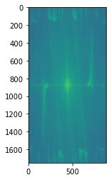
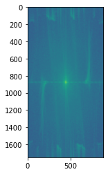
Of the above results, I find Figure 11 to be the most satisfying. The low pass filter sigma is 15 and the high pass filter sigma is 25. You can see the log magnitude of Fourier transform the two input images, filtered images, and hybrid image. Note that the filtered Bow has low frequencies and the filtered Luna has high frequencies compared to the originals. The hybrid has them combined.

Part 3: Multi-resolution Blending and the Oraple Journey

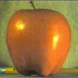
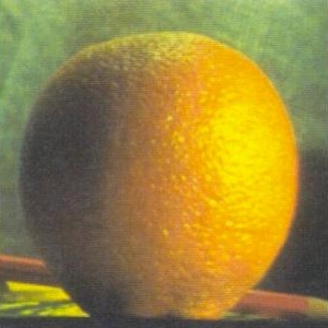
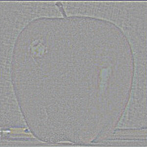
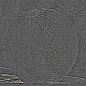
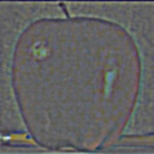
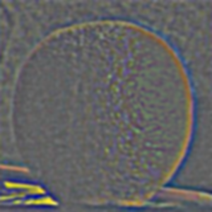
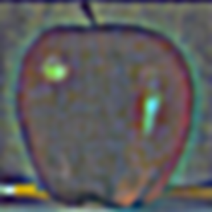
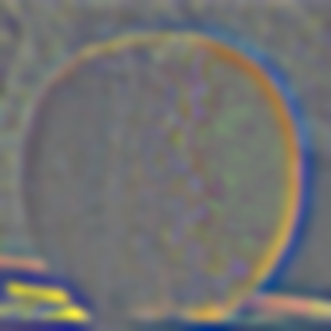
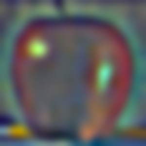
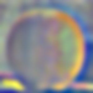
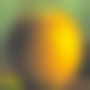
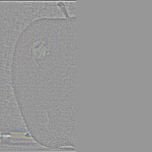
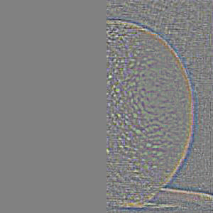
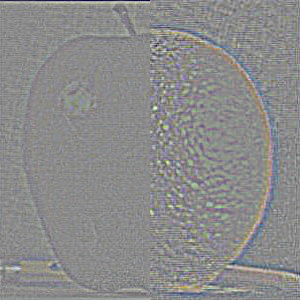
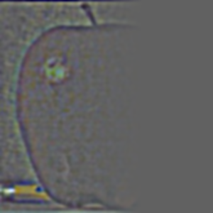
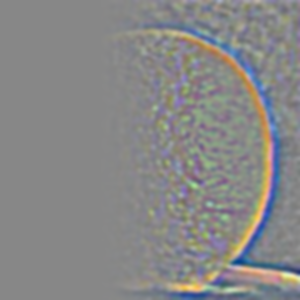
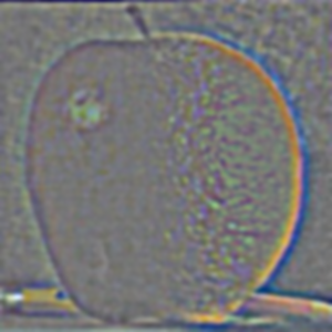
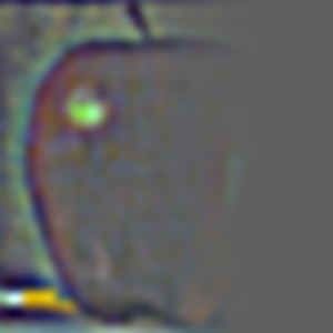
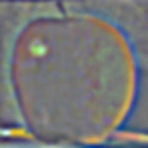
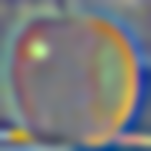
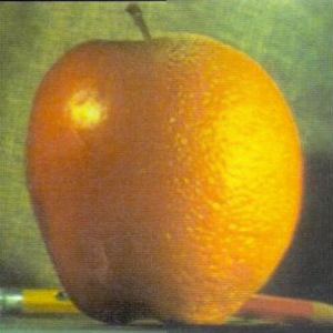
Every day we stray further from God's light by making some bizarre mixed images. In this part, we generate smooth blending with multi-resolution blending. In the first example, we blend an apple and an orange together. To do this, we make a Laplacian stack of both the apple and the orange. To do this, we create a Gaussian stack of each image. We convolve the image with increasingly blurrier kernels. Then we create the Laplacian band-pass layers by subtracting the layers of the Gaussian stack from each other.

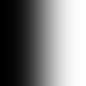
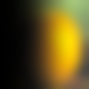
At the same time, we have a mask filter that we are using to select for certain parts of each image. In this case, we use a horizontal mask. This mask is also made into a Gaussian stack. They get progressively blurrier. Not that this is only one of the masks. The other half of the image is generated using 1-mask. The other mask is not visualized for neatness's sake.

From here, we can then multiply through each layer. At each layer, the mask is multiplied with the Laplacian image. The other mask is multiplied with the other Laplacian image. Then the images are summed together to form an complete image at each layer. Finally, all the images that were summed are collapsed into a final image.

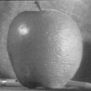
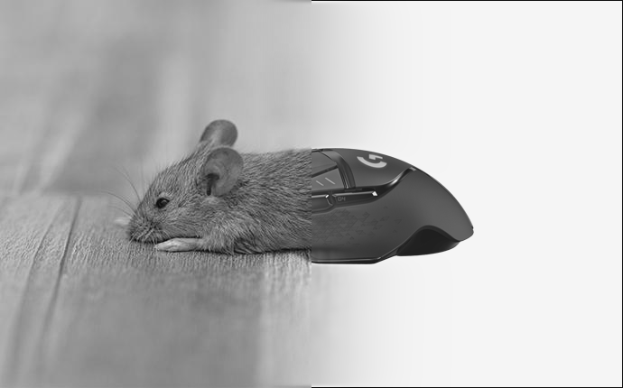
This works because we use the sharp filter on the sharp details, but the vast majority of the image is the low pass filtered images of the orange and apple. These are blurred across a large common space. This makes the blending look smooth. However, the sharper filters provide just enough detail on the edges to make it not look too blurry and instead look like one smooth seam. Below are the final results in color and greyscale. Note that the greyscale looks a bit smoother because there are fewer channels to coordinate.

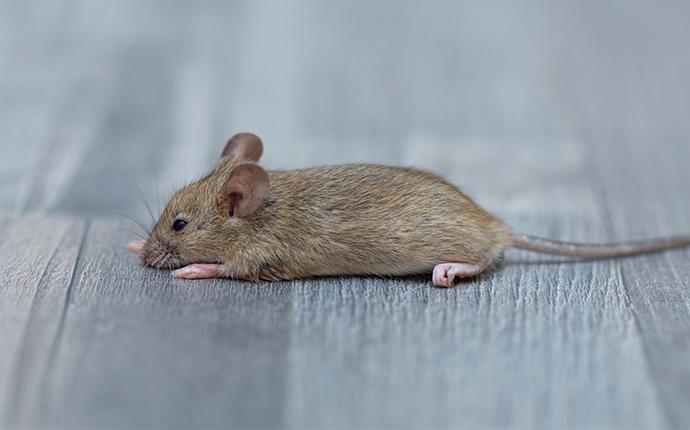
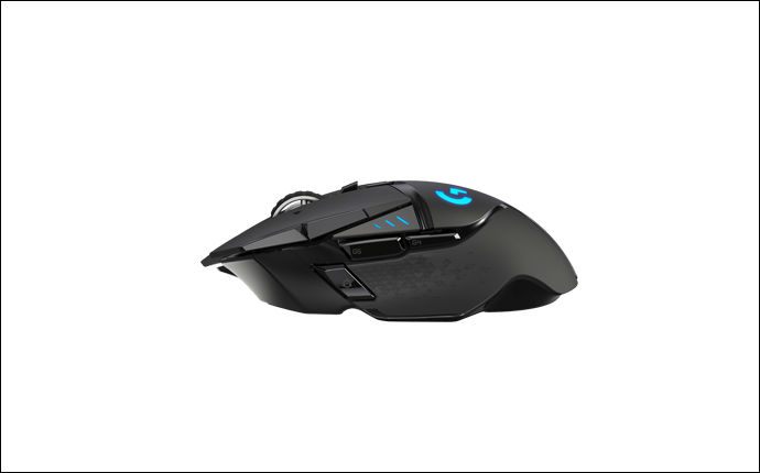
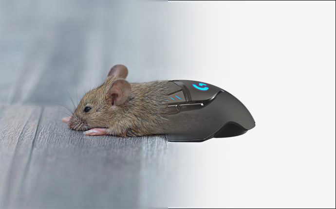
Using a similar style horizontal mask, we can create other things! Below is a visual pun. The transition is less smooth because of the high frequencies in the fur of the mouse. This makes the seam a little more difficult to smoothen, but you can tell by the background that it is blending smoothly. Additionally, you can see one of the blue ticks from the computer mouse make its way into the rodent's fur.

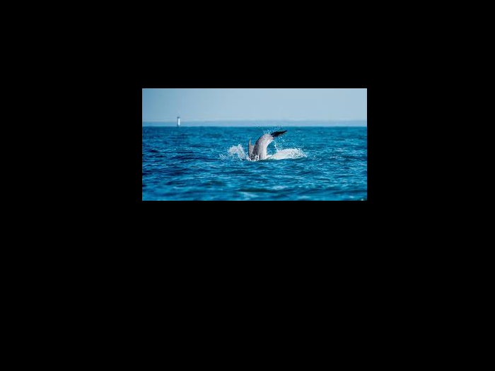
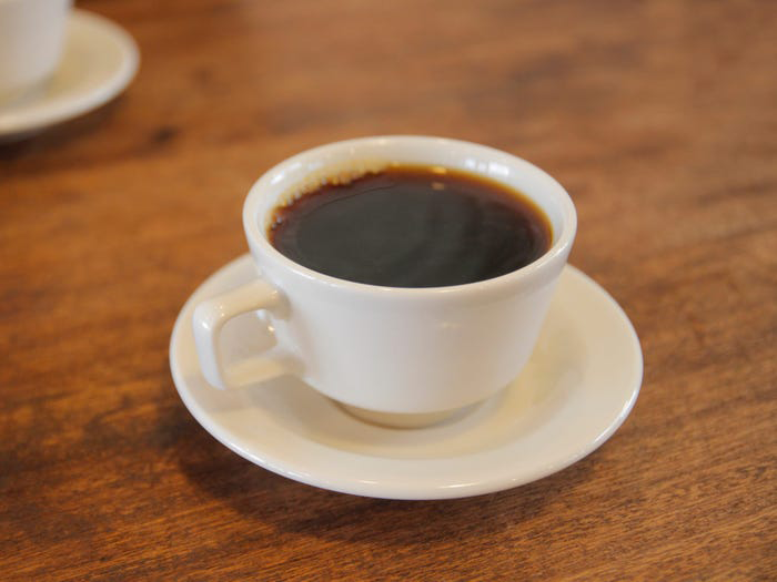
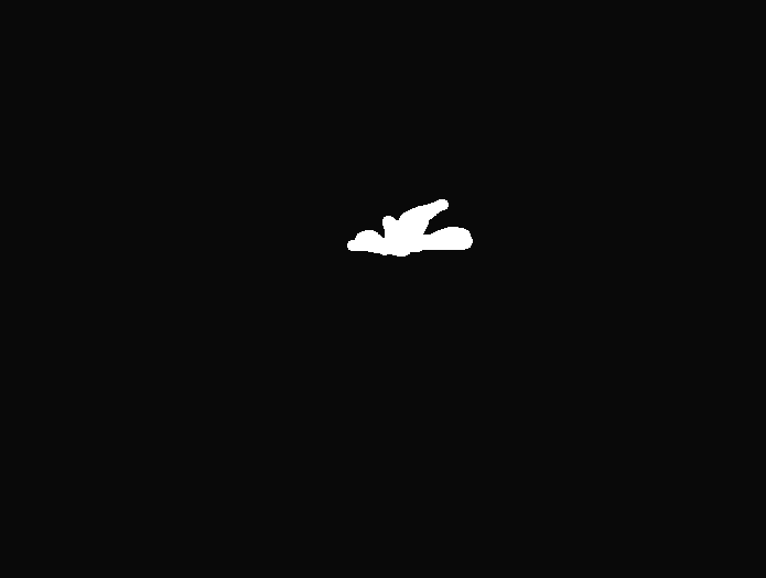
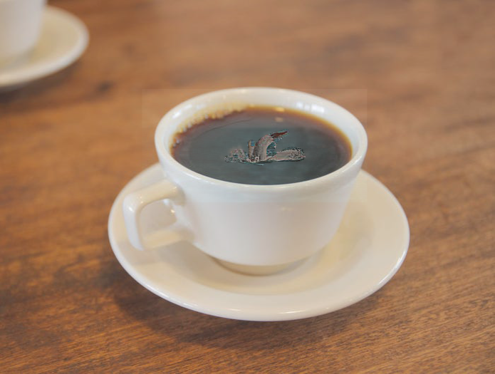
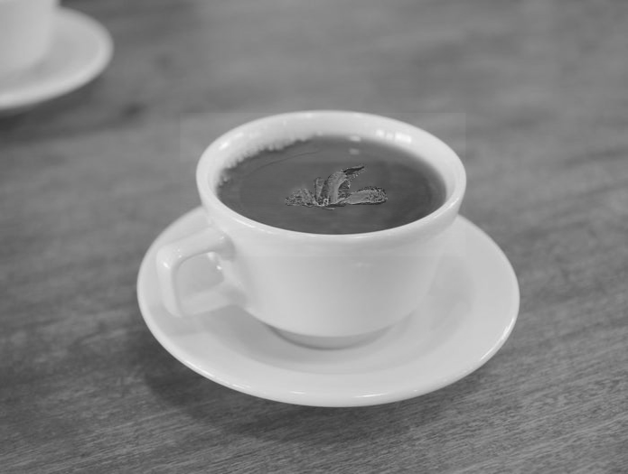
A fun thing to note is that the masks need not be just horizontal/vertical and in the middle. You can generate aribtrary masks. Below, we blended dolphins jumping out of coffee. Note that the image of the dolphin must be extended to match that of the coffee to maintain a reasonable scale for the dolphins to jump out.