Fun with Filters and Frequencies!
William Ren
1.1 Finite Difference Operator
To compute the gradient magnitude of an image, we first take the partial derivatives of the image in both the x and y directions. We approximate the partial derivatives by taking the intensity difference of adjacent
pixels, done by convolving the image with a finite difference operator [1, -1] in either the x or y directions (D_x or D_y). Once we calculate the partial derivatives of the image, we take the magnitude of the combined image to
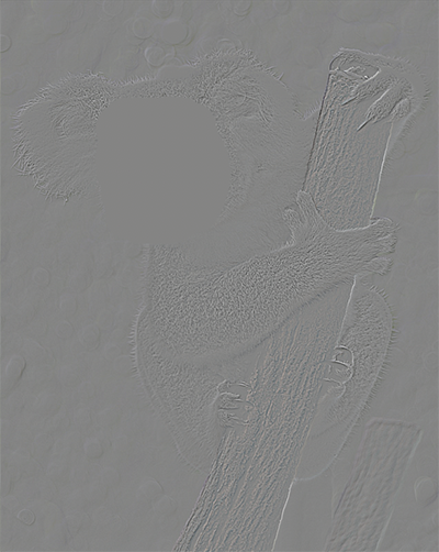
to get the gradient magnitude of the image. Since the magnitude is largest when there is a large change of intensity between adjacent pixels, we can use this process as edge detection. It is outlined in images below:
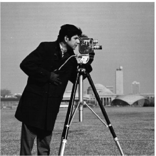 Original Image
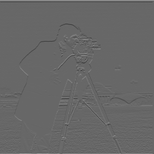
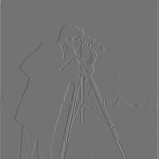 Original Image Convolved with D_x
|
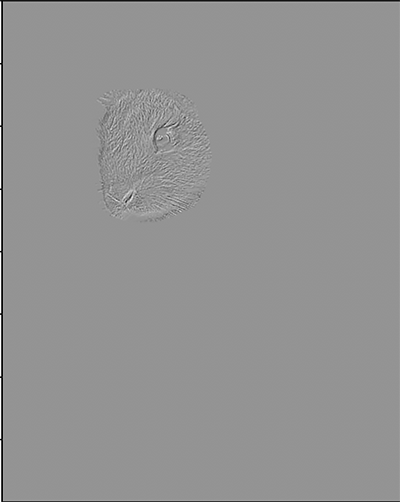
 Original Image Convolved with D_y
|
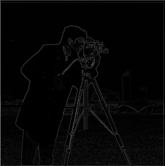 Gradient Magnitude
|
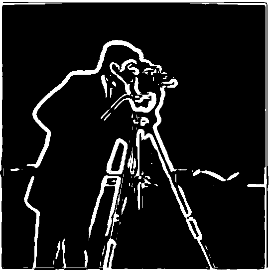
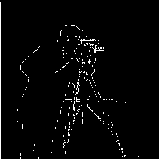 Binarized Gradient Magnitude
|
1.2 Derivative of Gaussian (DoG) Filter
Notice that the results from using the finite difference operator are rather noisy. To smooth the edges we detect, we can blur the original image by convolving it with a gaussian filter before performing convolutions with the finite difference operator.
Alternatively, we can also convolve the guassian filter with the finite difference operator to produce a derivative of gaussian filter, such that we only need to do a single convolution with the original image. As a result, we end up with these two filters:
 Derivative of the Gaussian in the X Direction
|
 Derivative of the Gaussian in the Y Direction
|
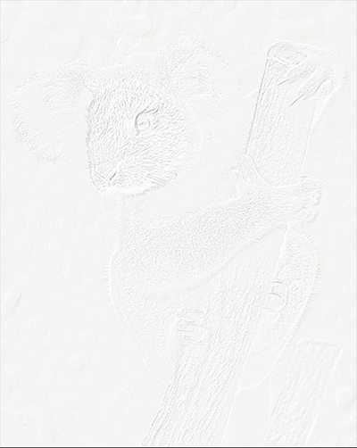
Both of these approaches produce smoother and less noisy edges compared to the prior results, as we can see from the images below:
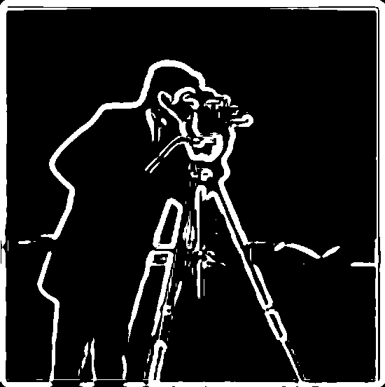 Original Image Convolved with the Derivative of Gaussians Filter
|
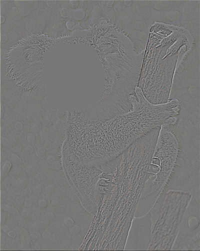
 Same Results Using the Alternate Approach
|
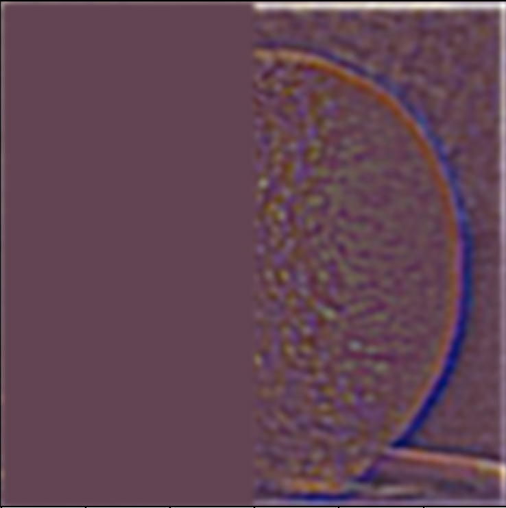
2.1 Image "Sharpening"
We can convolve images with an unsharp mask filter to sharpen them. We create the unsharp mask filter by subtracting the gaussian filter from the unit impulse. Essentially, what we are doing is subtracting the blurred image from the original. Doing so removes
the low frequencies from the image, only leaving behind high frequencies that produce sharp edges. By adding these high frequencies scaled by a value of alpha to the original image, we can effectively sharpen the original image. Some results are shown below:
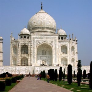 Original Taj Mahal Image
|
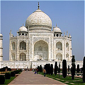 Taj Mahal Sharpened with the Unsharp Mask Filter
|
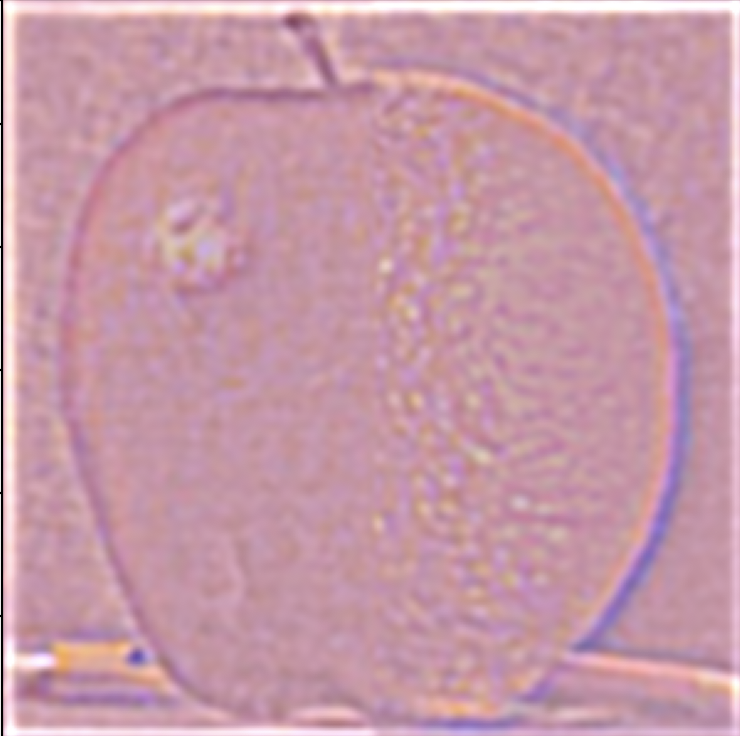
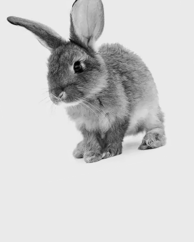
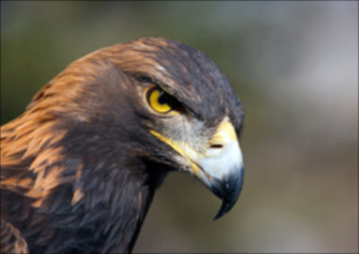
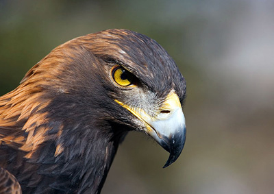 Original Eagle Image
|
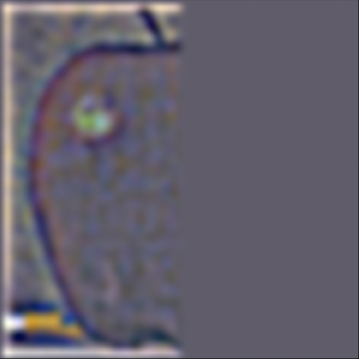
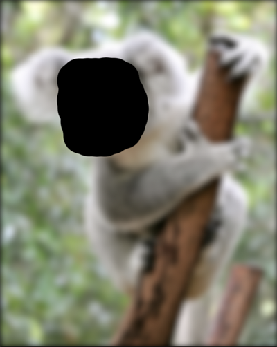
 Blurred Eagle Image
|
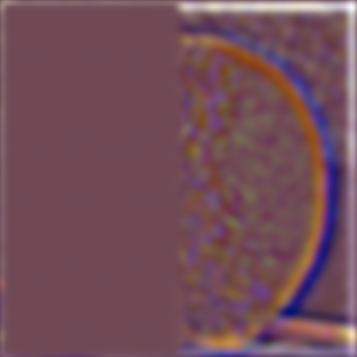
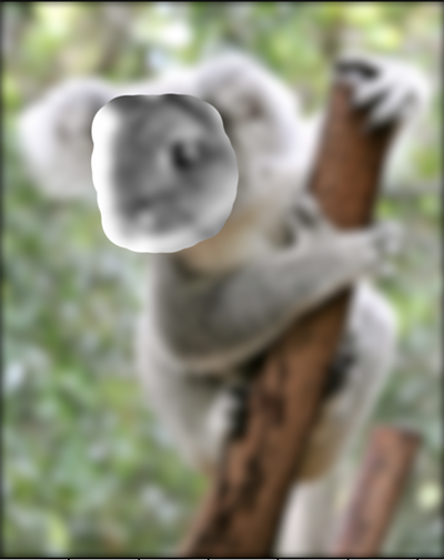
 Sharpened Blurred Eagle Image
|
The bottom sequence of pictures illustrates my process of taking an image, blurring it, and then sharpening the result. Sharpening the blurred picture to look similar to the original took a higher alpha value compared to a non blurred image. In addition, the
result is not the exact same as the original image. Since blurring the image removes a lot of the high frequencies in the original image, those frequencies can not be reconstructed purely from sharpening the image.
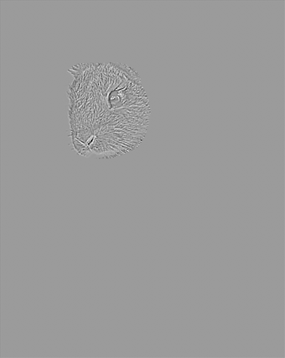
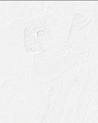
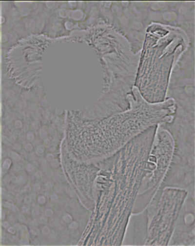
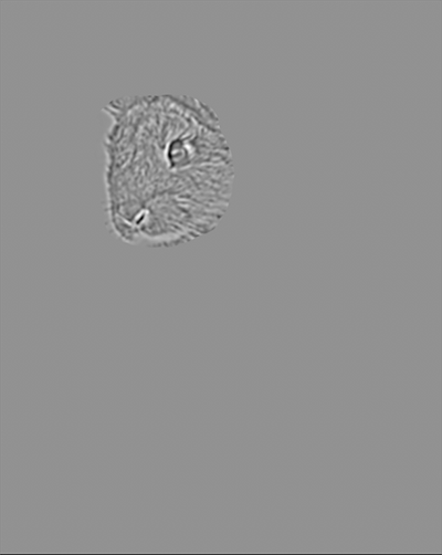
2.2 Hybrid Images
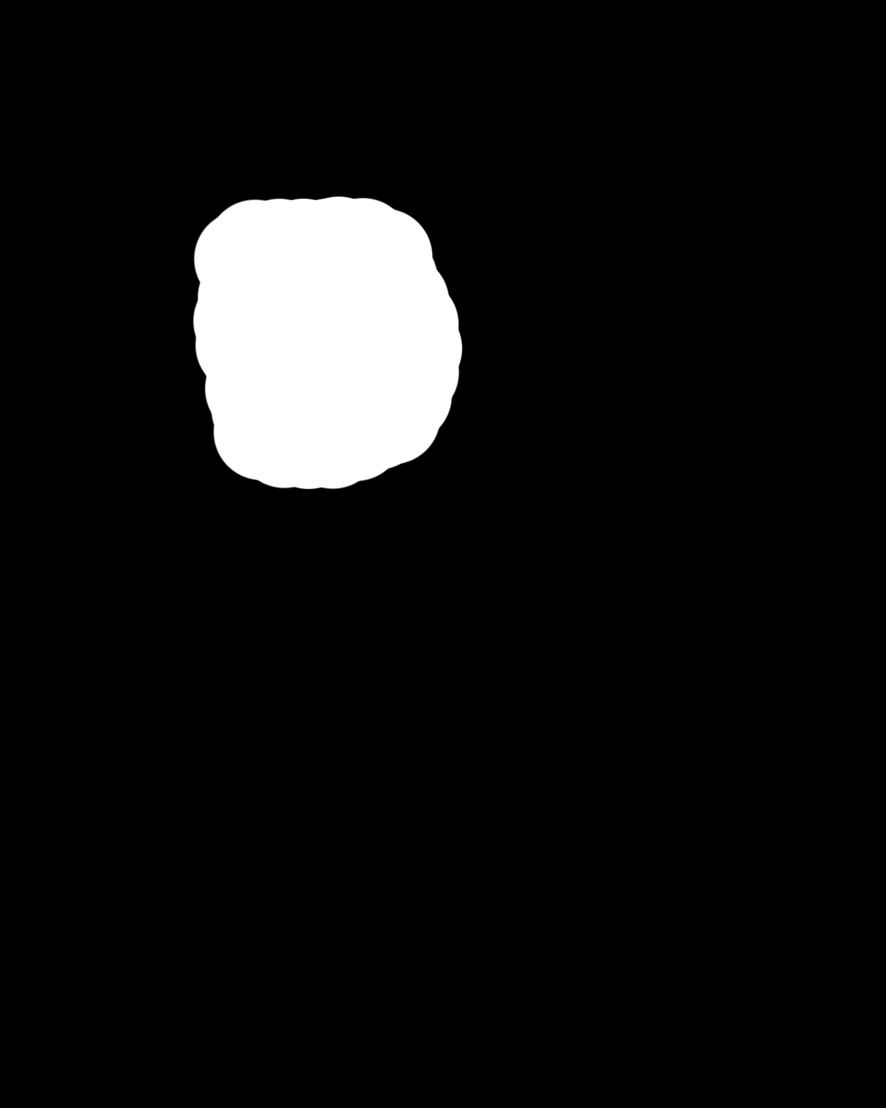
The hybrid images we create are essentially two images overlaid on top of each other, where the image appears different depending on how close you are to the image when viewing it. To achieve this effect, we apply a high pass filter to one image and a low pass filter
to the other. The low pass filter will make the image seem blurry such that it is indiscernable close up, while the high pass filter will only keep sharp details that are only apparent when viewing the image up close. The provided alignment code is used to align the
images around some chosen anchor points. A few results are shown below:
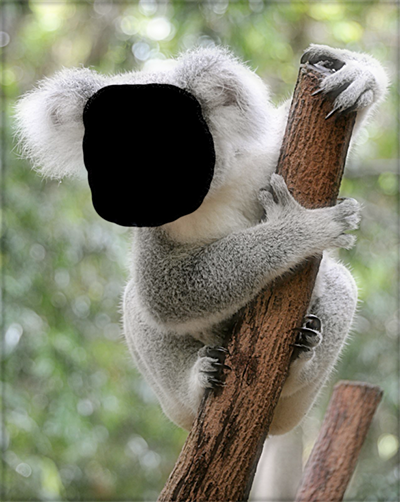
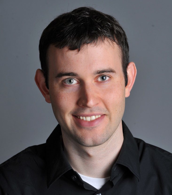 Original Image of Derek
|
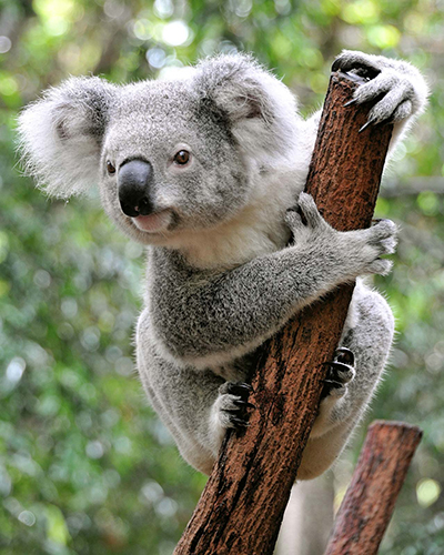
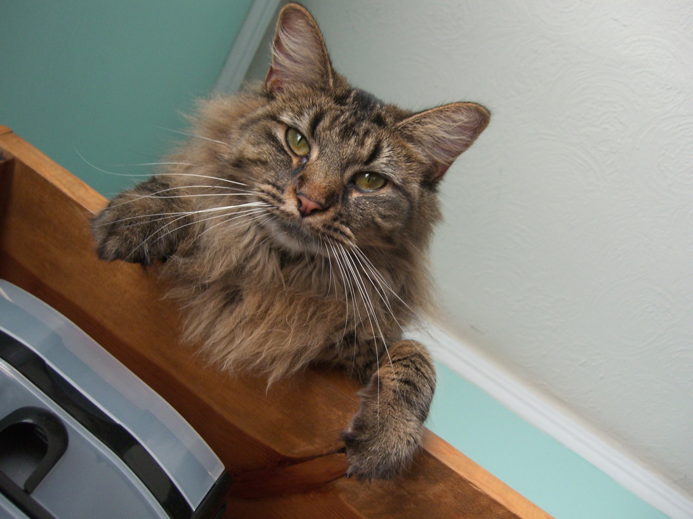 Original Image of Nutmeg
|
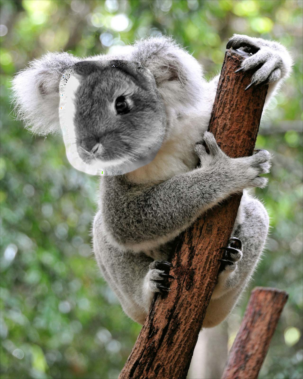
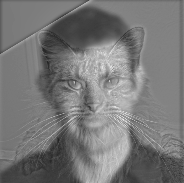 Derek Nutmeg Hybrid
|
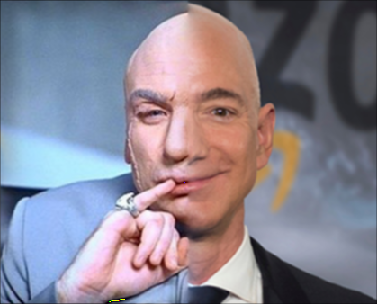
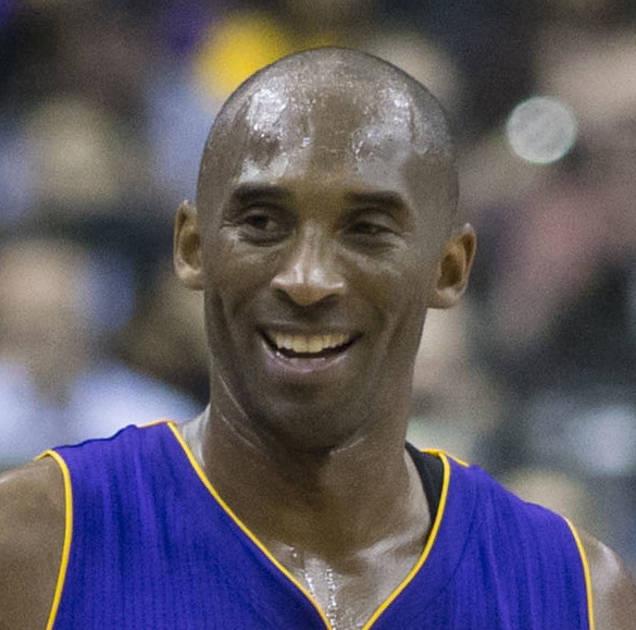 Original Image of Kobe Bryant
|
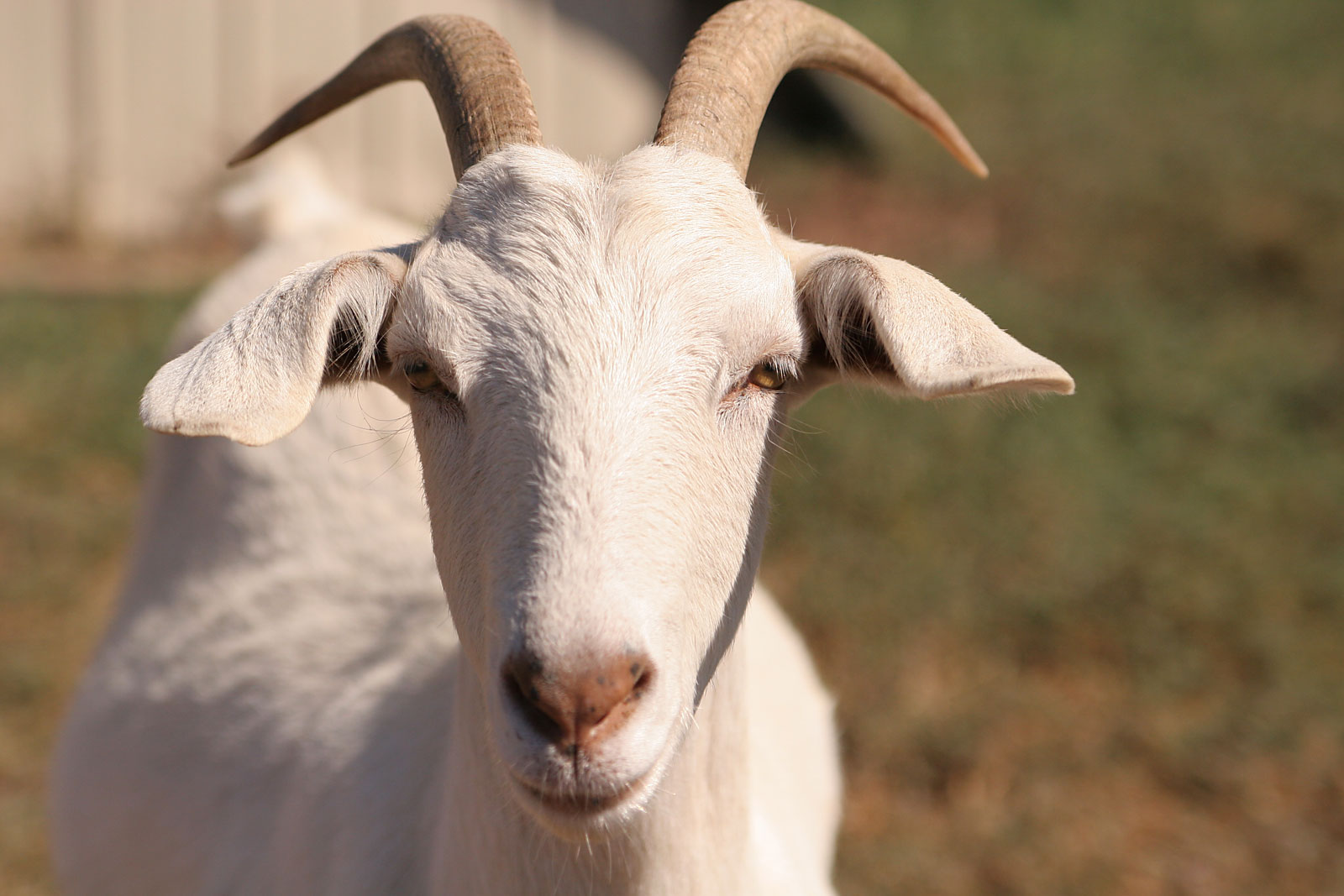 Original Image of a Goat
|
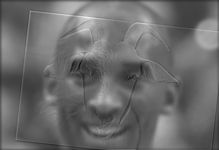 Kobe is Goated
|
Notice that the second example is not great. While Kobe is the GOAT, the hybrid image does not reflect it very well since it was difficult to align the goat's face and Kobe's. After all, their eyes are
located in significantly different places on their respective head. We get much better results when 'hybridizing' two more similar images, which we can see below. The images below also illustrate this
process in the frequency domain:
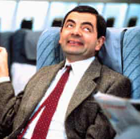 Original Image of Mr. Bean
|
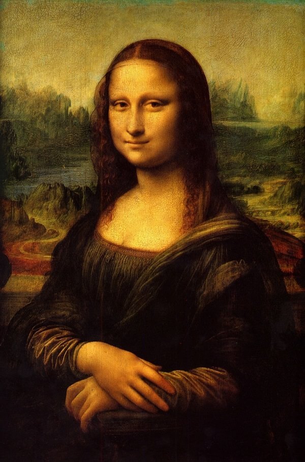 Original Image of the Mona Lisa
|
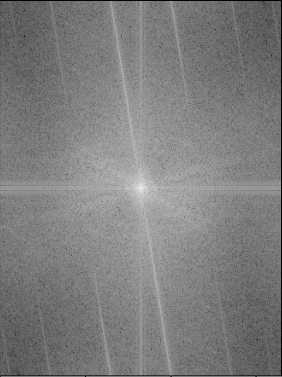
 Mr. Bean in Fourier Space
|
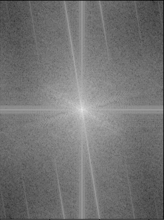
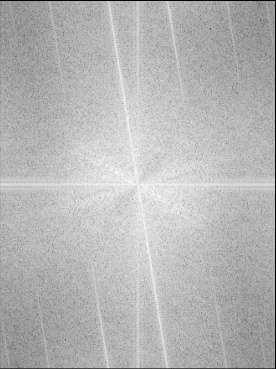
 Mona Lisa in Fourier Space
|
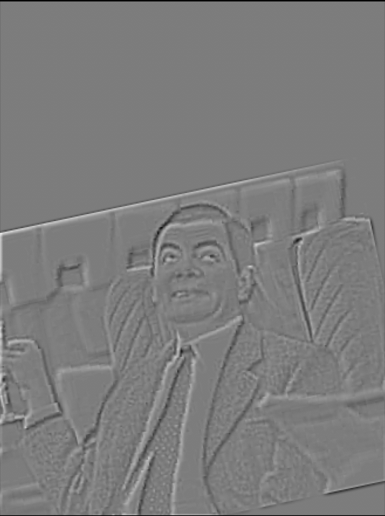 High-Pass Filtered Mr. Bean
|
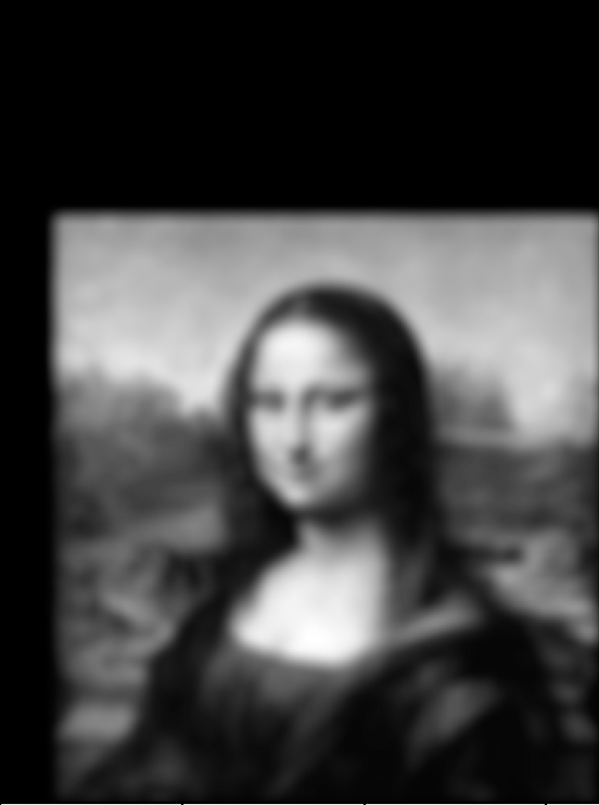 Low-Pass Filtered Mona Lisa
|
 High-Pass Filtered Mr. Bean in Fourier Space
|
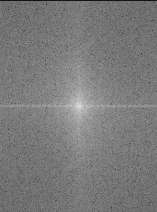
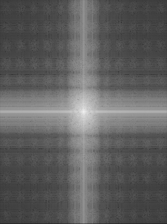 Low-Pass Filtered Mona Lisa in Fourier Space
|
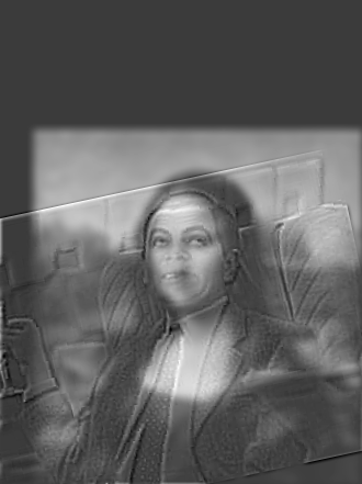 Mr. Bean and Mona Lisa Hybrid
|
 Hybrid in Fourier Space
|
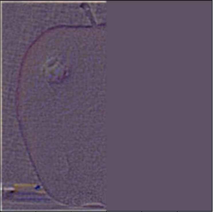
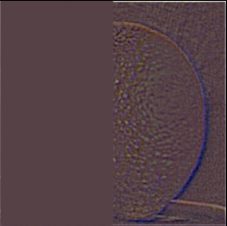
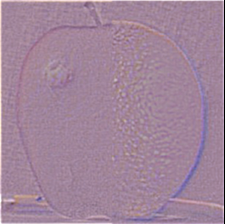
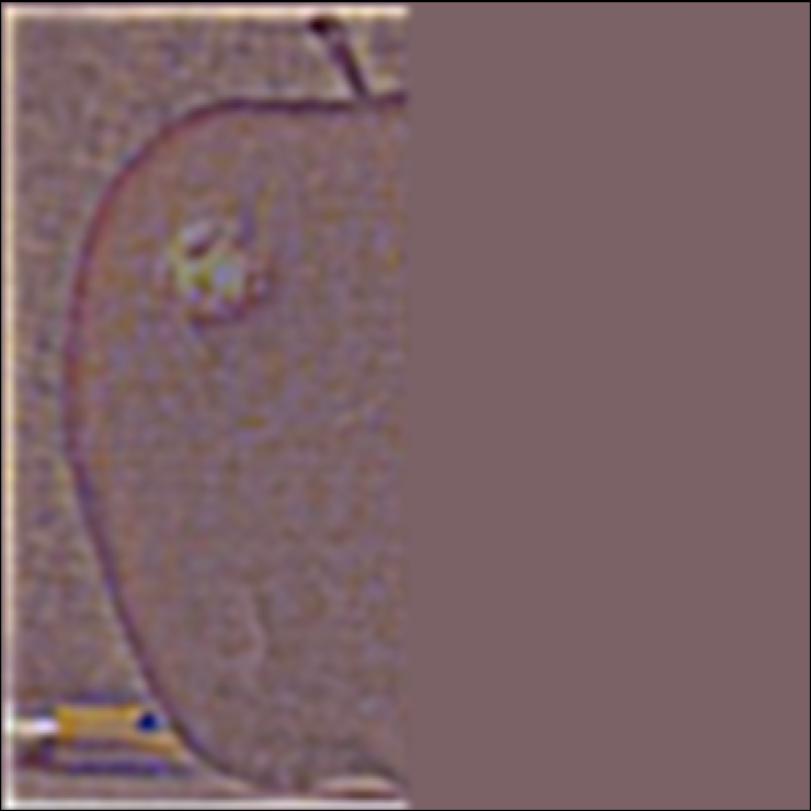
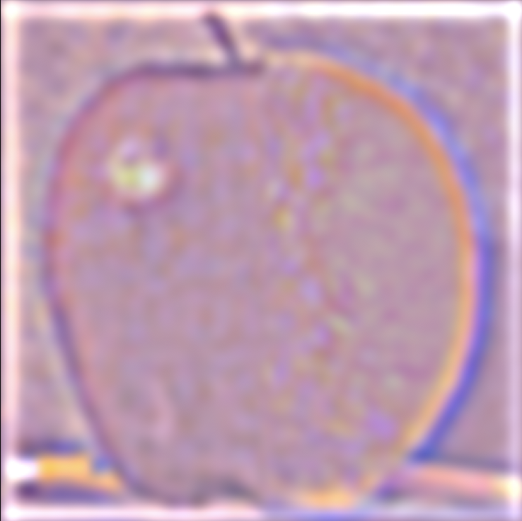
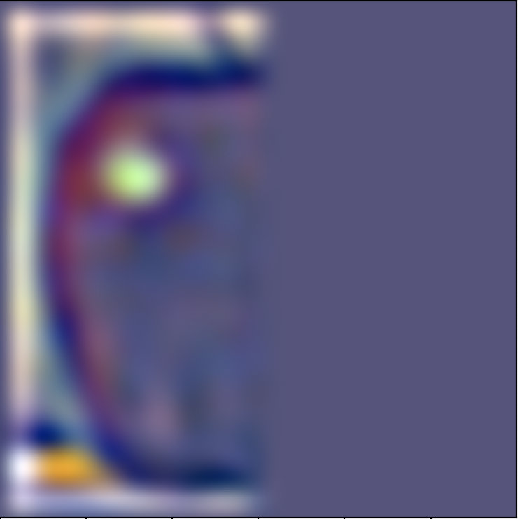
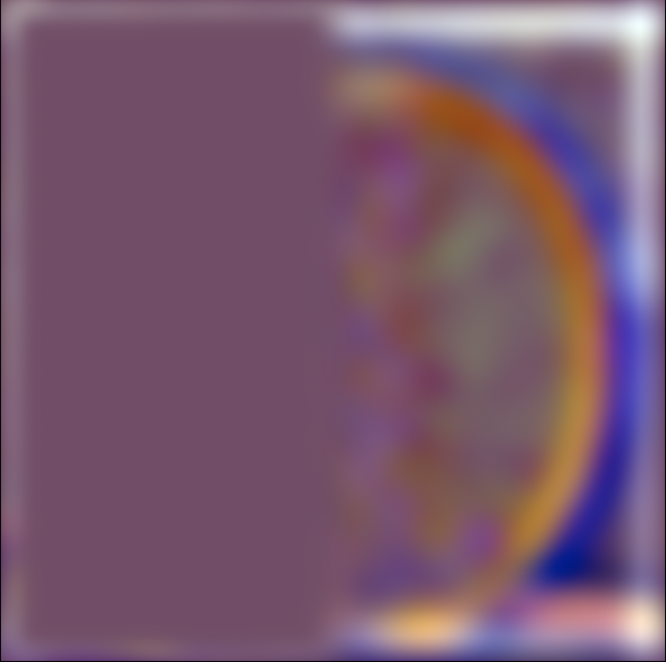
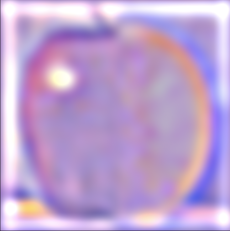
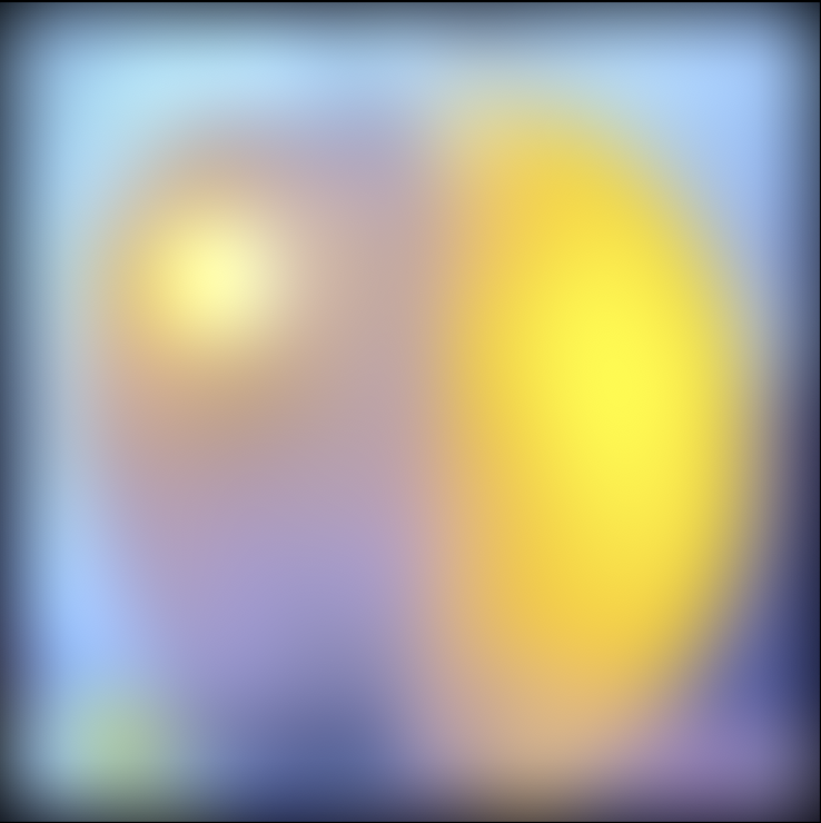
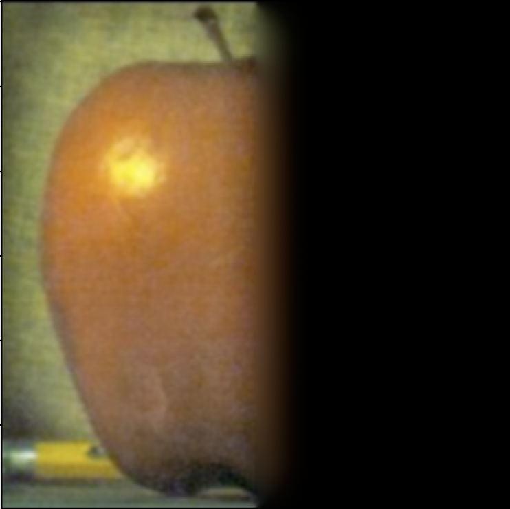
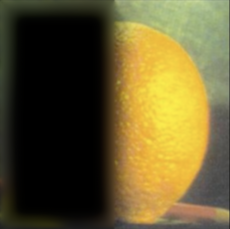
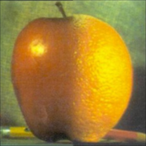
2.3 Gaussian and Laplacian Stacks
In this subpart we implement Gaussian and Laplacian stacks to be used for multiresolution blending. To create a Gaussian stack, we repeatedly convolve an image with a gaussian filter, resulting in multiple same sized images
with different levels of clarity. We then create Laplacian stacks from these Gaussian stacks, where each layer Laplacian stack contains the difference between two adjacent gaussian stacks. As such, we get n-1 layers of a
Laplacian stack from n layers of a Gaussian stack. We then set the last layer of the Laplacian stack to be the same as the last layer of the Gaussian stack. With these stacks implemented, we are able to recreate the outcomes
illustrated in the original paper, which were Laplacian stacks corresponding to the blended oraple: