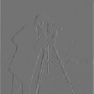
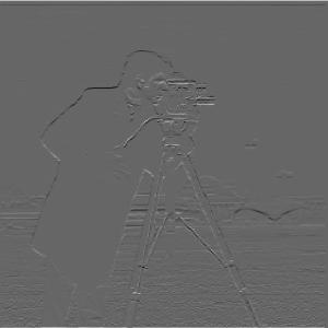
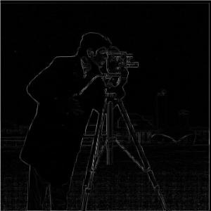
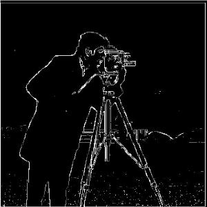
Given the original image of cameraman, the results obtained by convolving with dx, dy kernels are shown below. The gradient image is obtained by taking g=sqrt(px^2+py^2), where px and py are the pixels from the images convolved with a dx and a dy kernel, respectively. After adjusting the threshold for binarization (threshold=51 in my implementation), the edge images is shown below
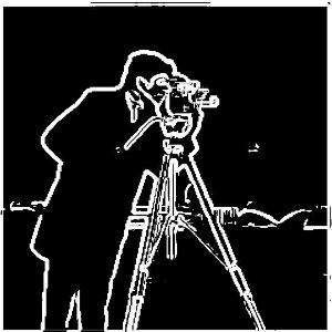
The previous edge image result seems to be a little noisy, and applying Gaussian filters before taking the derivatives helps smooth the results. The result obtained by first filtered by a Gaussian filter then the process of the previous subsection is shown below. The result obtained by applying Gaussian filter first produces stronger and smoother edges as well as less noisy pixels.
Since convolution operations are linear, we can simply combine the convolution kernels, i.e., take the dx and dy derivatives of gaussian filter to obtain a DoG filter, then apply the image with the DoG filter. The image of an DoG filter and the results obtained by convolving with a DoG filter is shown below. Apparently, the results obtained by DoG filter is identical to the previous one. In my implementation, I use a Gaussian kernel with size=7 and sigma=5, and the threshold for binarizing the edge image is adjusted to 10.


In my implementation, I tried a Gaussian kernel with size=7 and sigma=1 as a low-pass filter. The sharpened results can be obtained by first subtract the Gaussian blurred image as a high frequency part and then add the high frequency to the original image, which can be formulated as sharp_image=(1+alpha)*origin_image-gaussian_image (alpha=2 in my implementation). Since convolution operation is linear, this can also be done by convolving with a single kernel, which can be obtained by (1+alpha)*impulse_kernel-gaussian_kernel, where a impulse kernel is a kernel with 0s except at the central point. Results of the example image is shown below. In addition, to prevent `skimage.io.imsave` from rescaling the image which cause the images to be grayer than it should be, the images are clipped to [0, 1].
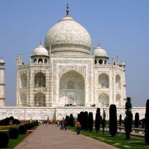
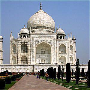

The chosen image is shown below.
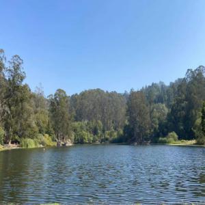
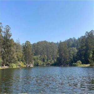
The results for first blur the image by Gaussian kernel and then recover by image sharpening is shown below. However, the image could not be fully recovered since there is information loss in the low-pass filtering process.
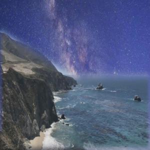
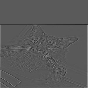
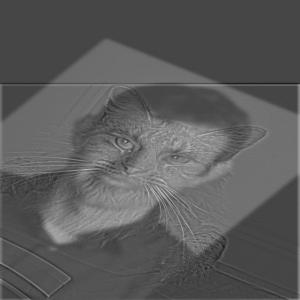
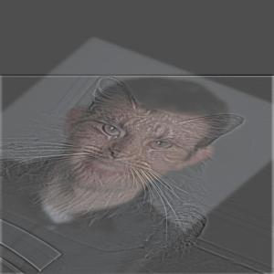
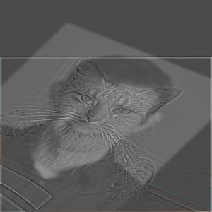
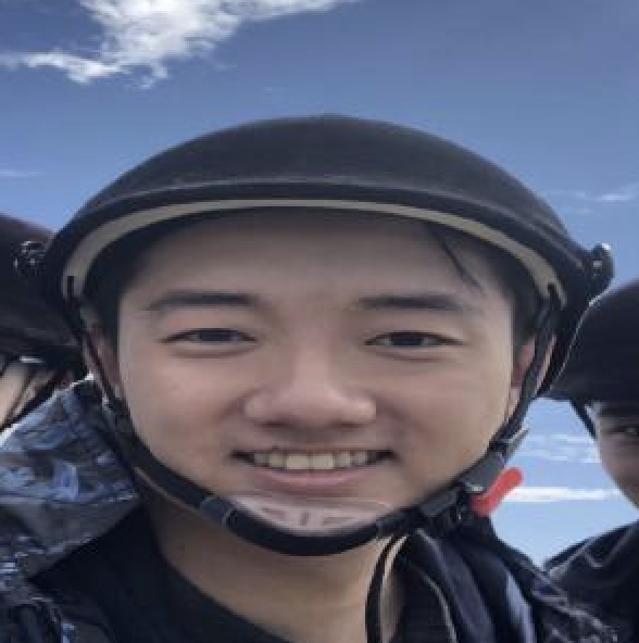
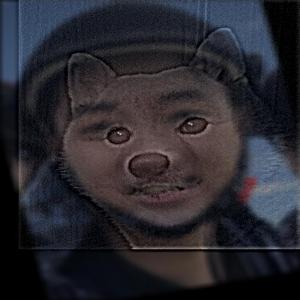
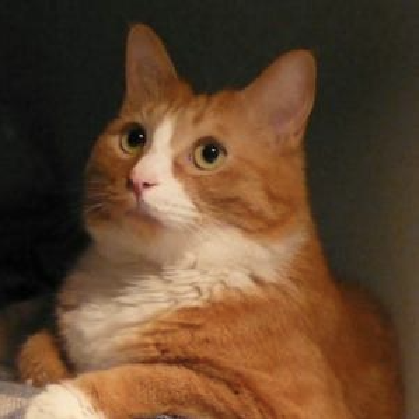
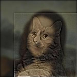
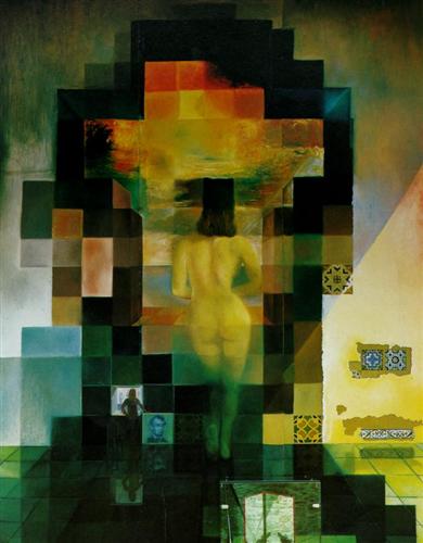
To create a hybrid image, one of the image is low-pass filtered so that the blend image should look similar to it from a far distance, and the other is high-pass filtered. In my implementation, I used Gaussian kernel of size=17 and sigma=17 for low-pass filtering and impulse kernel subtracted by that Gaussian kernel for high-pass filtering. The blend image is the summation of alpha*high-frequency part and the low-frequency part (alpha=3 in my implementation). The result of the example image in grayscale is shown below.
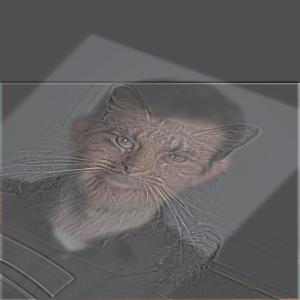
Results of introducing color to the above example is shown below. I tried three different approaches to introduce color: keep the color of the blur image, keep the color of the sharp image, and keep the color of both. Keeping the blur image colored produces better results, while keeping only the sharp image colored seems to have little difference from the grayscale (except that the eyes are a little colored). Also, comparing to the grayscale blend result, the color of the blur image tends to guide human perception to recognize the blend object as human more than a cat.
Thus, it is hard to say whether using color works better, since color can guide people to better discriminate the subtle object which balance the saliency of the two objects, producing better blend images; meanwhile color can also mislead to more attention on the salient part, causing the saliency between the two unbalanced and producing a bad blend image.
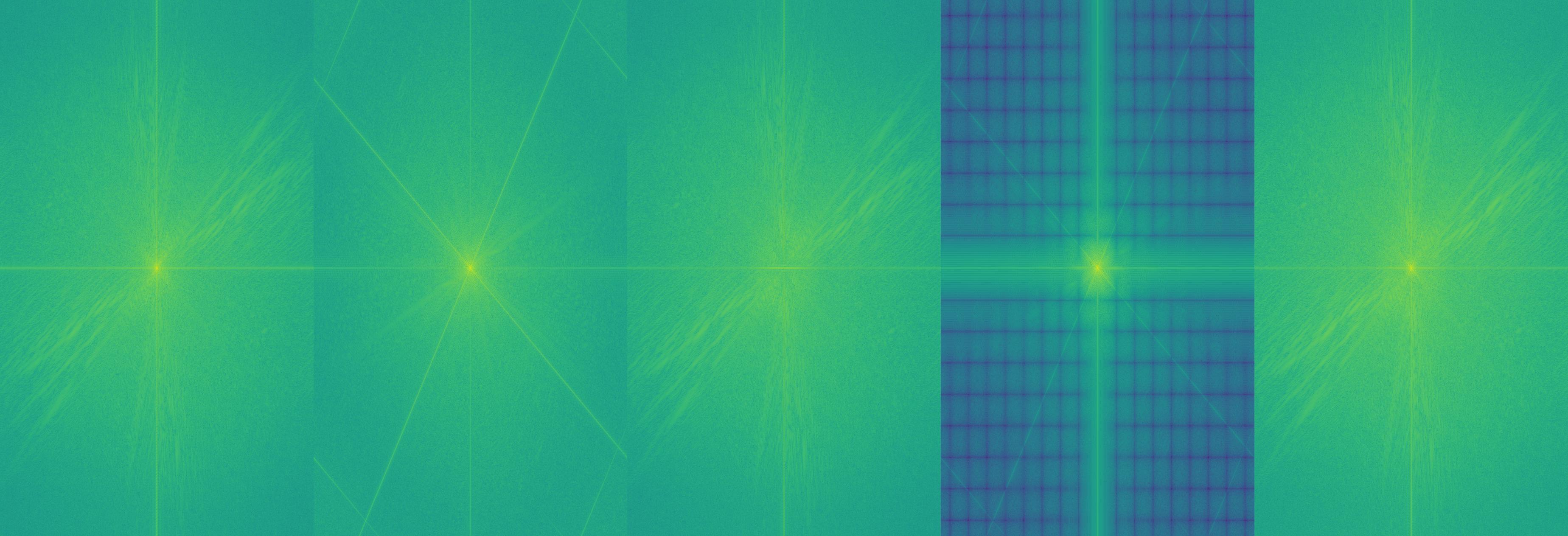
The Fourier image of the above result by keeping both colored is shown below. Apparently, the high frequency components of the sharp image is added to the low frequency components of the blur image.
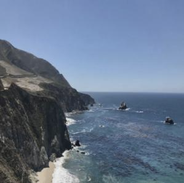
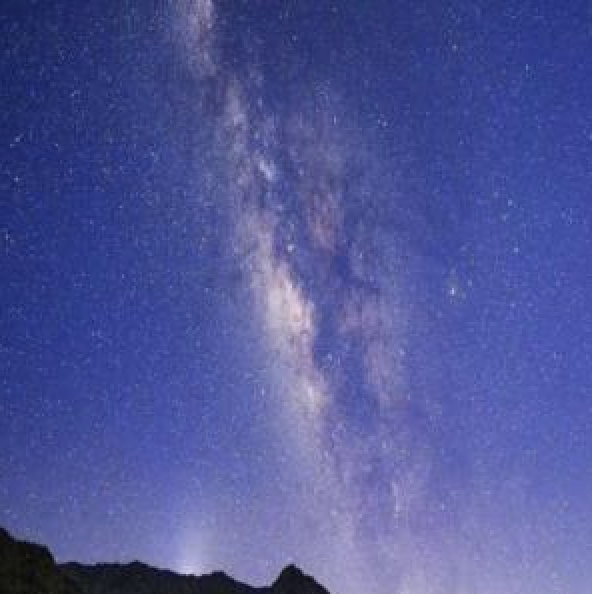
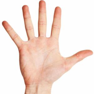
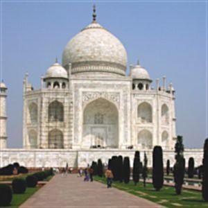
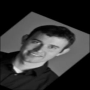
Here are some pictures of my choice!

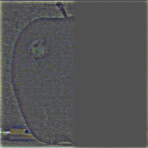
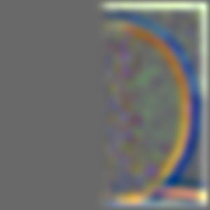
For this part, I used a Gaussian kernel of size=17, sigma=5, and the depth of the stacks is 5. The laplacian stack is generated by using the previous level image subtract the next level image in a Gaussian stack. The Gaussian and Laplacian stack of the following image is shown below.
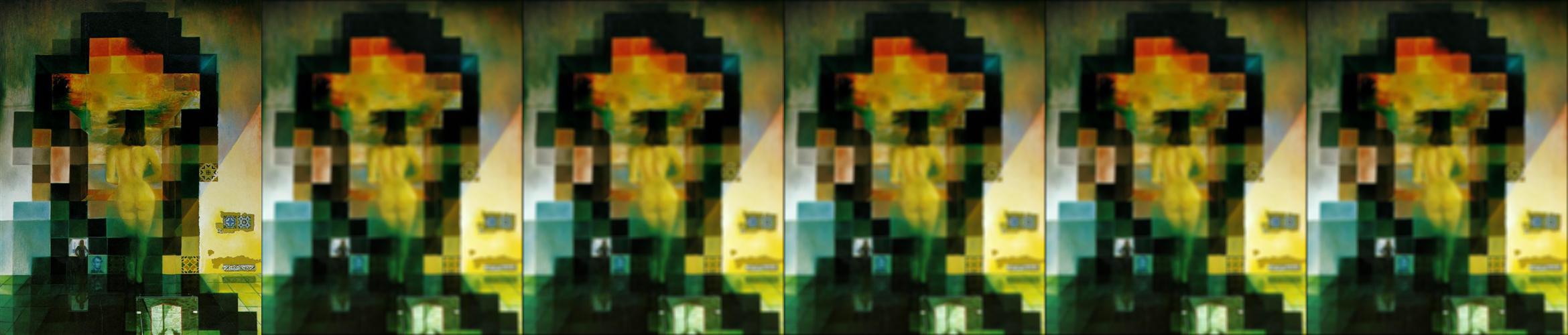
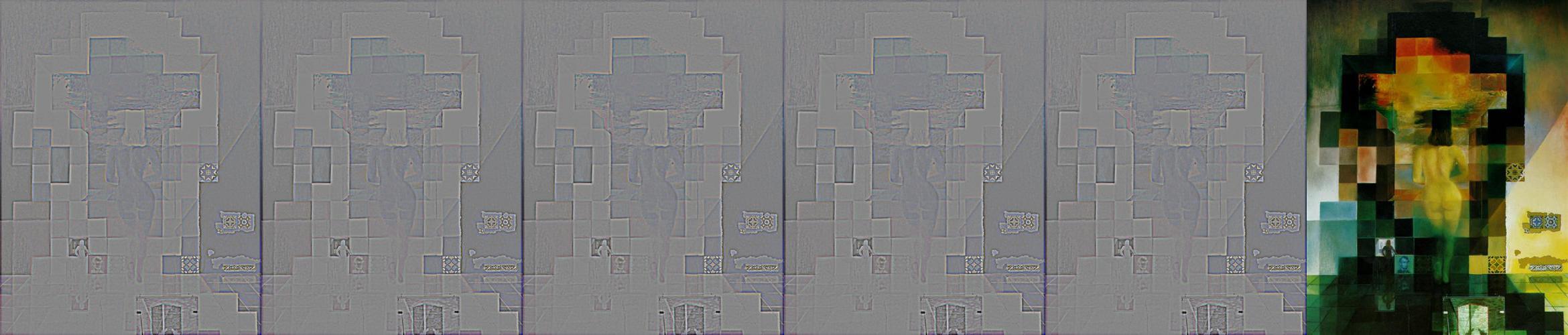
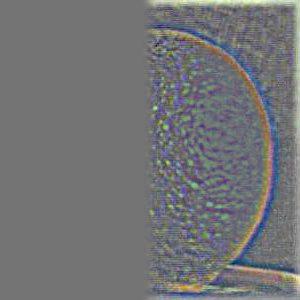
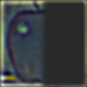
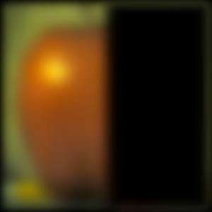
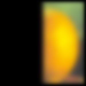
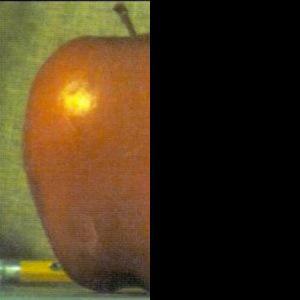
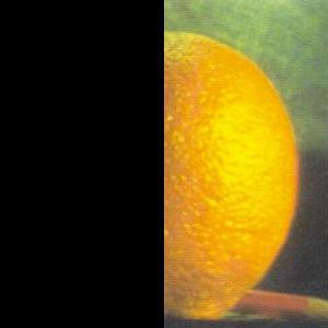
Results of the high, mid, low frequency parts of the oraple is shown below.
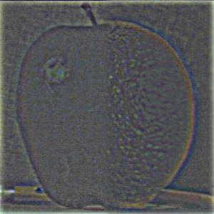
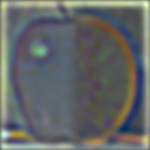
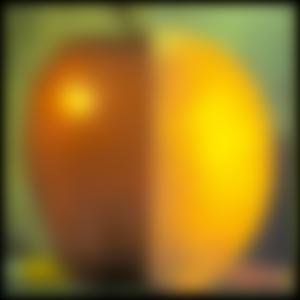
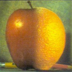
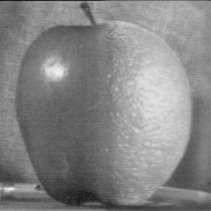
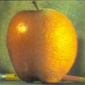
For this part, I used exactly the same parameters as in section 2.3 except that the depth of stacks becomes 30, which requires more computation but also yields better results. The gray and colorful oraple result is shown below.
The result of using depth=30 stacks blends better at the details that the boundary between is apple and the orange is more vague. Using colorful images actually enhance the effect, since the transition of color is smoother, while the transition in grayscale is relatively sharp and apparent.
Here are some other images of my own.