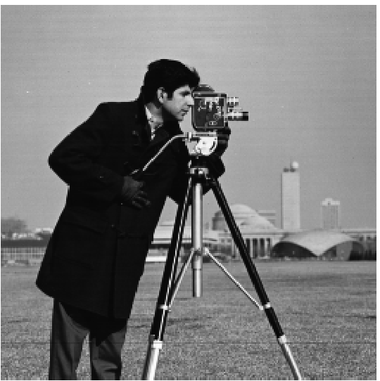
The goal is to compute the gradient magnitude of an image. The following details several approaches.
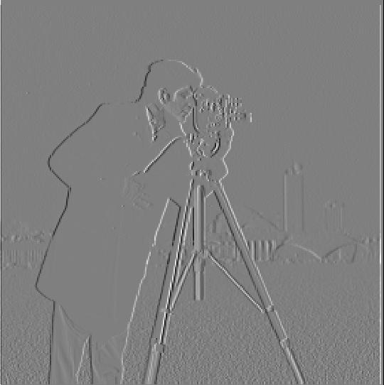
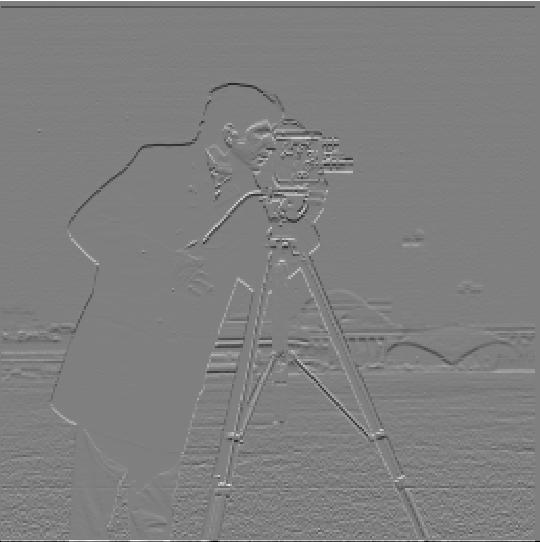
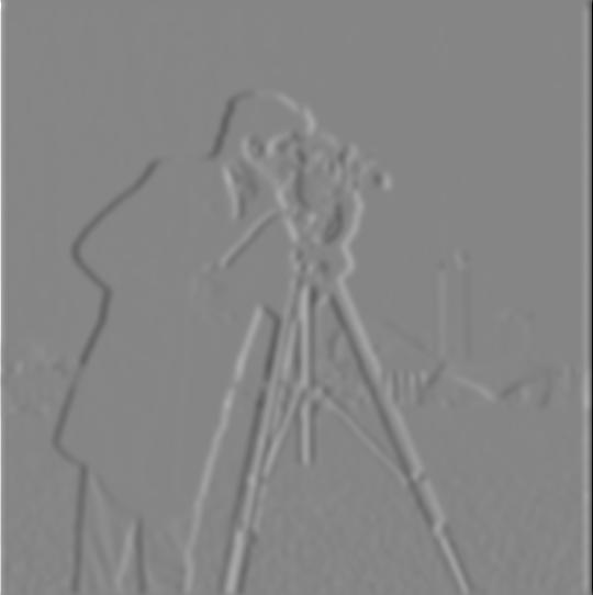
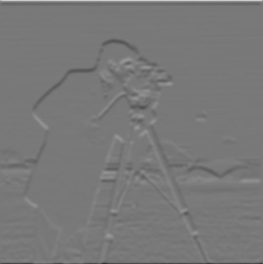
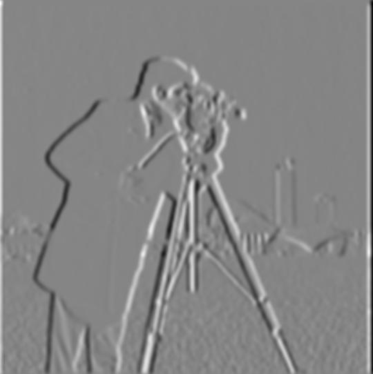
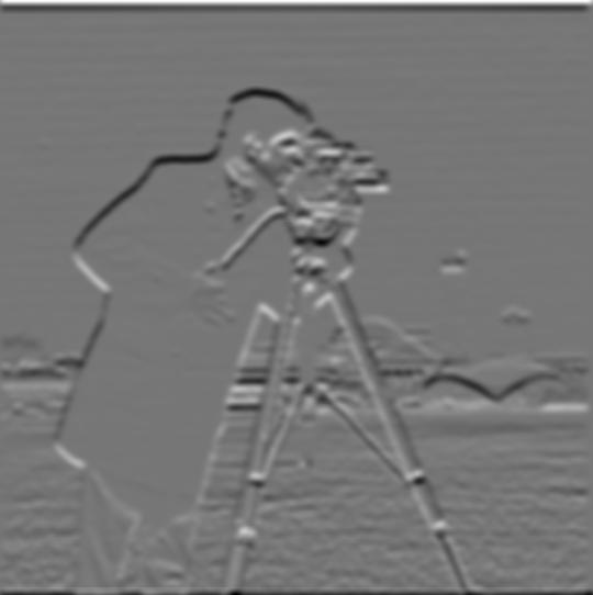
The first way is to obtain the partial derivatives of an image in both the x and y directions. We do this by convolving the images with the difference operators D_x and D_y.

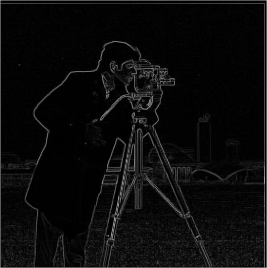
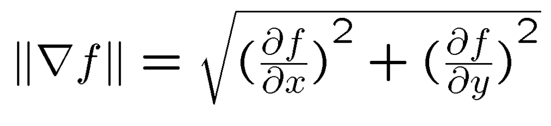
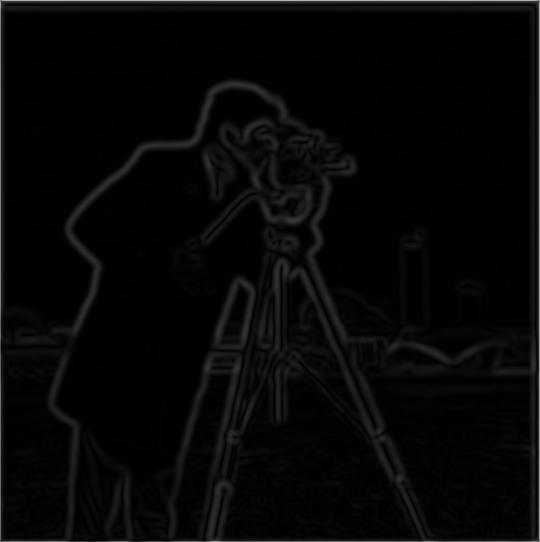
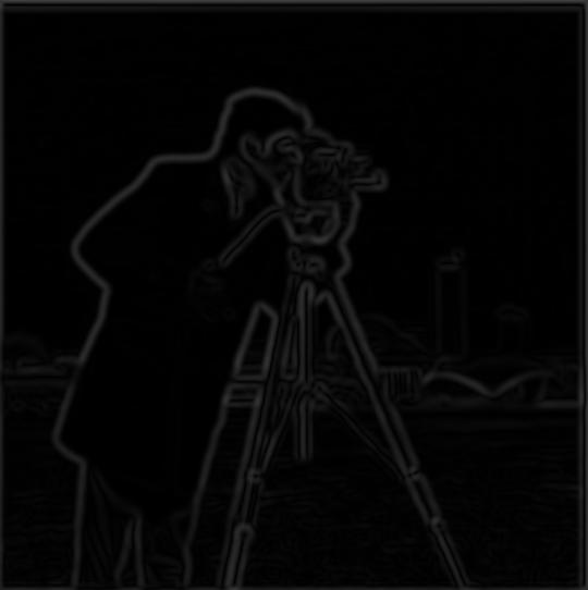
Then, we use the partial derivatives of the image to calculate the gradient magnitude.
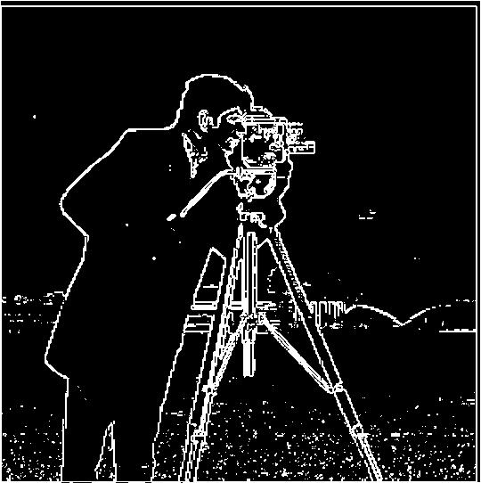
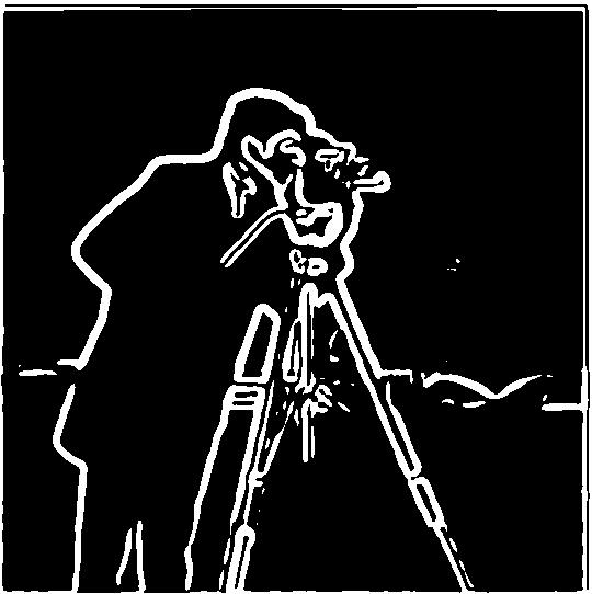
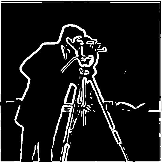
We can also obtain the edge image by binarizing the gradient magnitude. In the following example, I used a threshold of 0.18
Observe that the edge image above contains noise. Since we would like to reduce the amount of noise, we can blur the original image by convolving it with a Gaussian filter, G, prior to performing the steps in Part 1.1. This time, I use a threshold of 0.07 for the binarized gradient magnitudes.
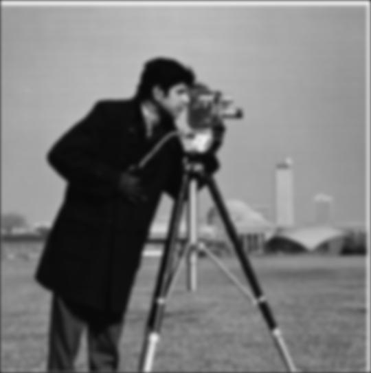
Now, the edge image is less noisy.
However, we can actually reduce the amount of computations without sacrificing the quality of our edge image.
Above, we needed to convolve the image with the Gaussian as well as each partial derivative. To reduce the number of convolutions as well as to be able to reuse the filters, we can pre-convolve the difference operators with the Gaussian. Then, we can also reuse these Derivative of Gaussian (DoG) filters on other images.


As expected, this edge image result is the same as before.
By boosting an image's high frequencies, we are able to artificially sharpen the image. The high frequencies can be computed by subtracting the low frequencies from the original image. Again, we use a Gaussian filter to blur the image and obtain the low frequencies.
We can combine these steps into a single convolution operation called the unsharp mask filter, which takes in a parameter alpha. This parameter, alpha, is the scaling factor for the high frequencies, and it determines how sharp the image becomes. For example, convolving an image with an unsharp mask filter of alpha = 0 gives us back the original image while using higher alphas gives us increasingly sharper images.
Below are several examples of "sharpened" images.
For 'timessquare.jpg' and 'storefront.jpg', the originals are first blurred, and then the sharpening is performed on the blurred images.
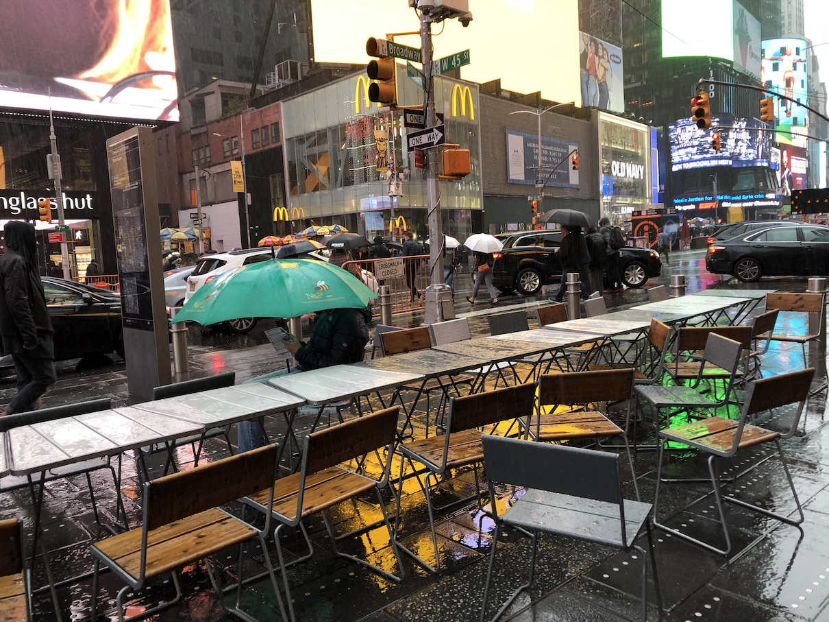
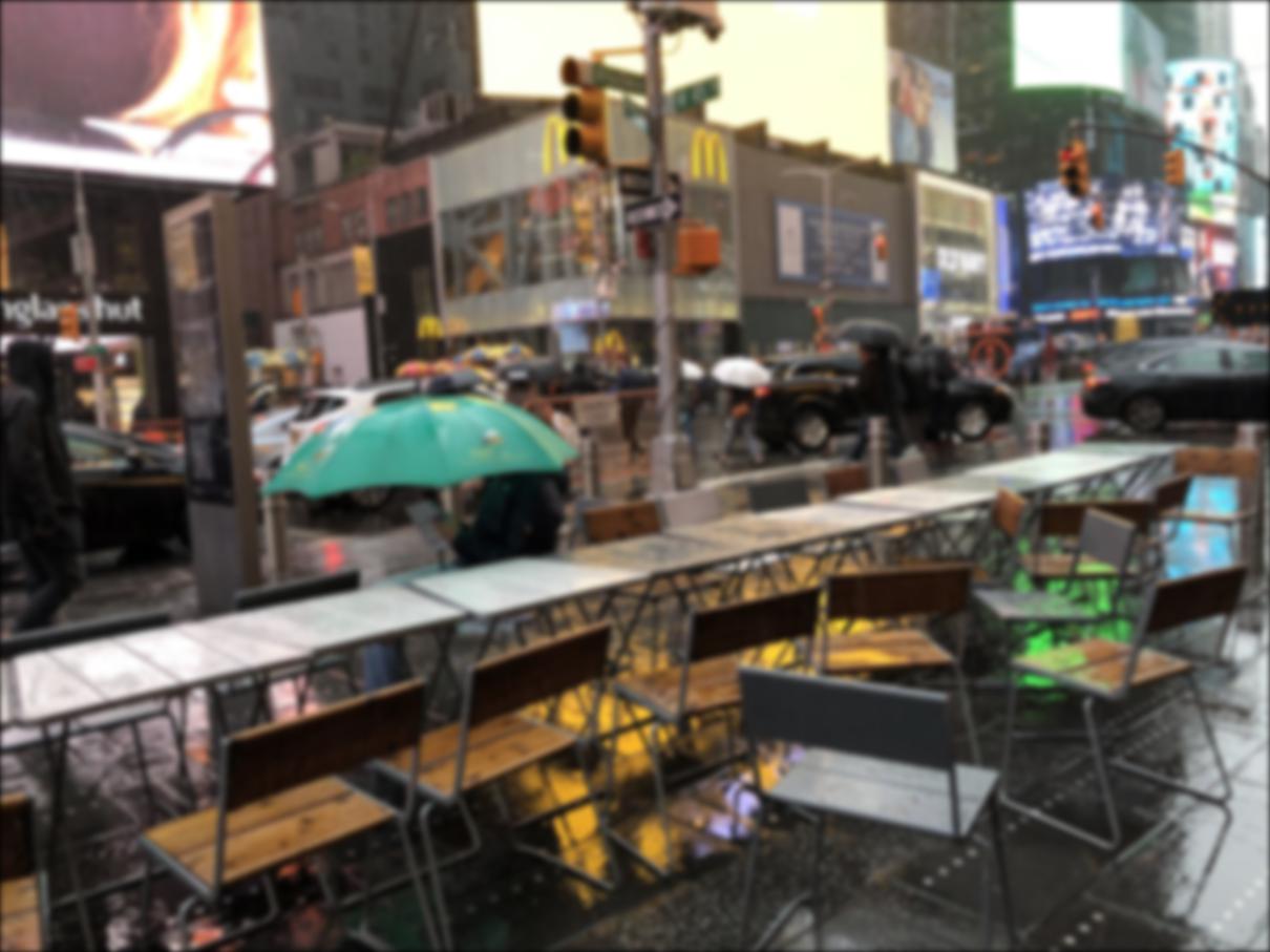
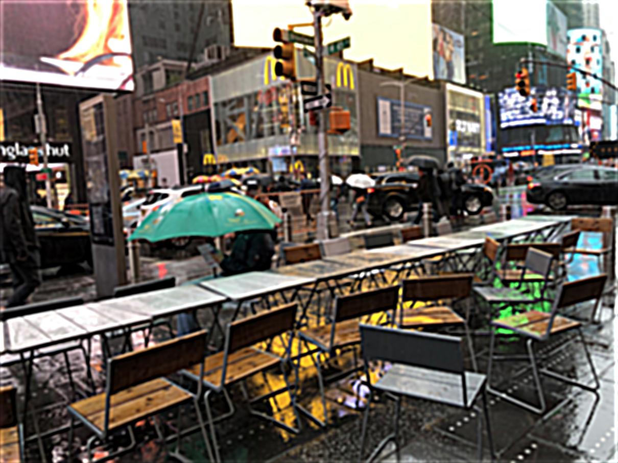
Image Credit: Hyacinth
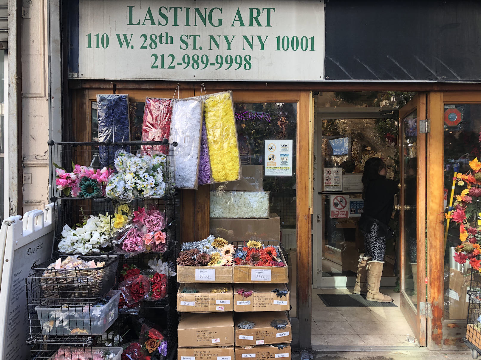

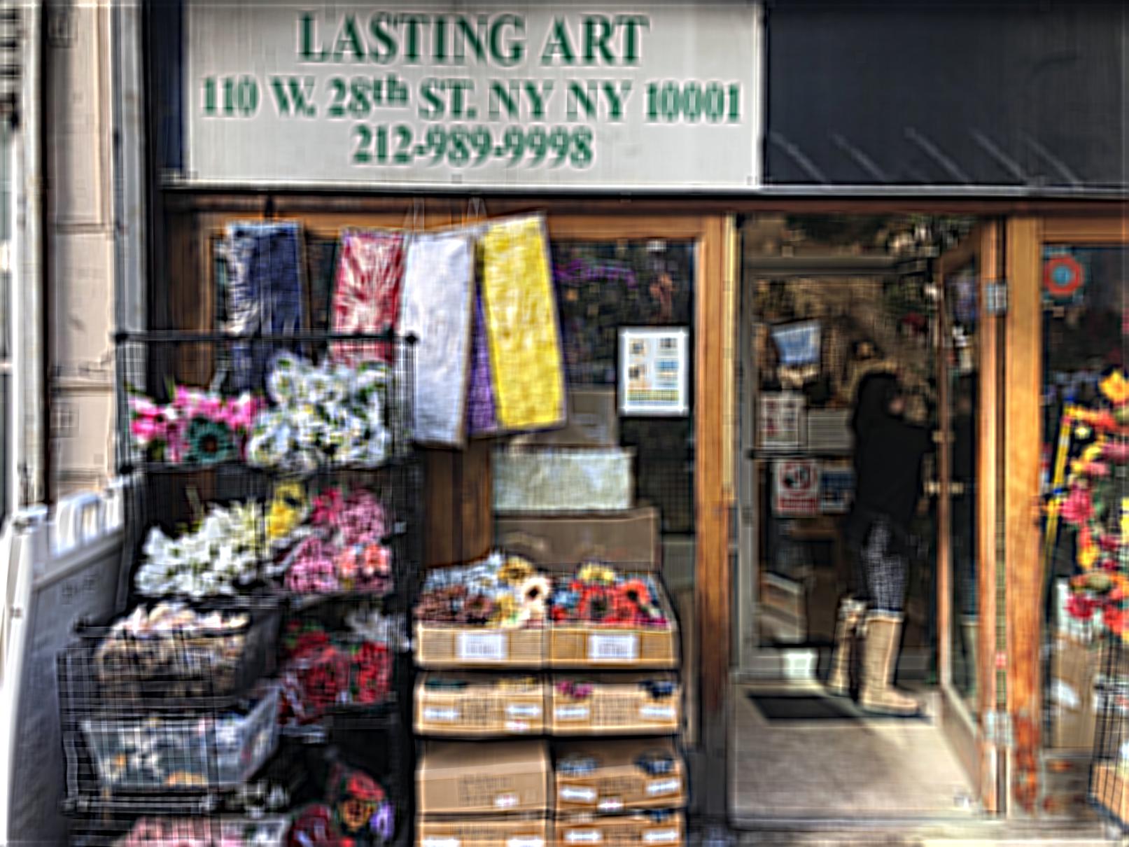
Image Credit: Hyacinth
"Look! Down below! It's a mouse! It's a mouse! It's...both!"
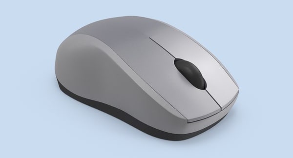
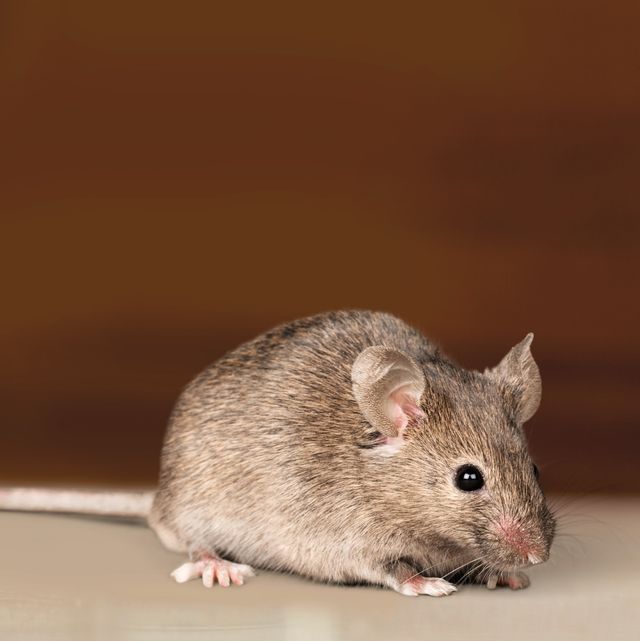
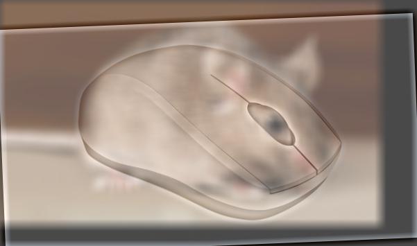
We can take advantage of the limits of human visual perception and create hybrid images in which the viewer sees one image up close and a different image far away. This is achieved by adding together the high frequencies of one image and the low frequencies of another. At close distances, the human eye is able to pick up the high frequencies, but at far away distances, the human eye can't perceive the high frequencies and only picks up the lower frequencies.
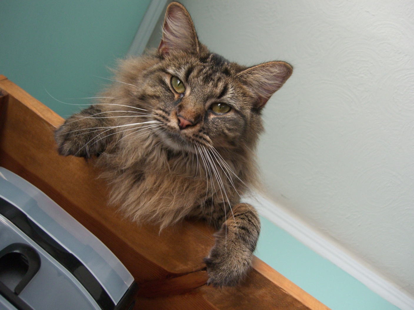
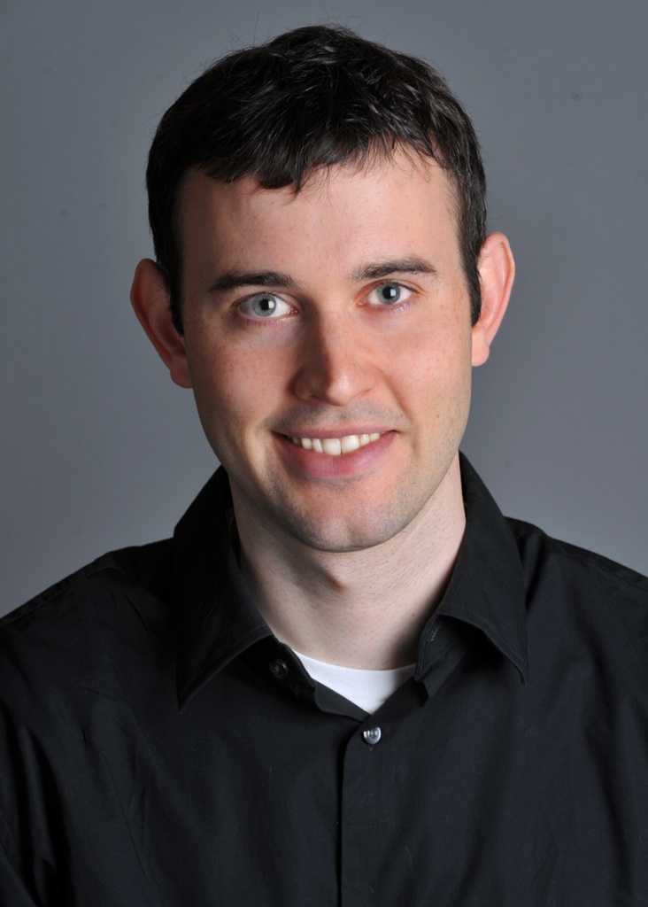
For example, below, you will see Nutmeg up close and Derek far away.
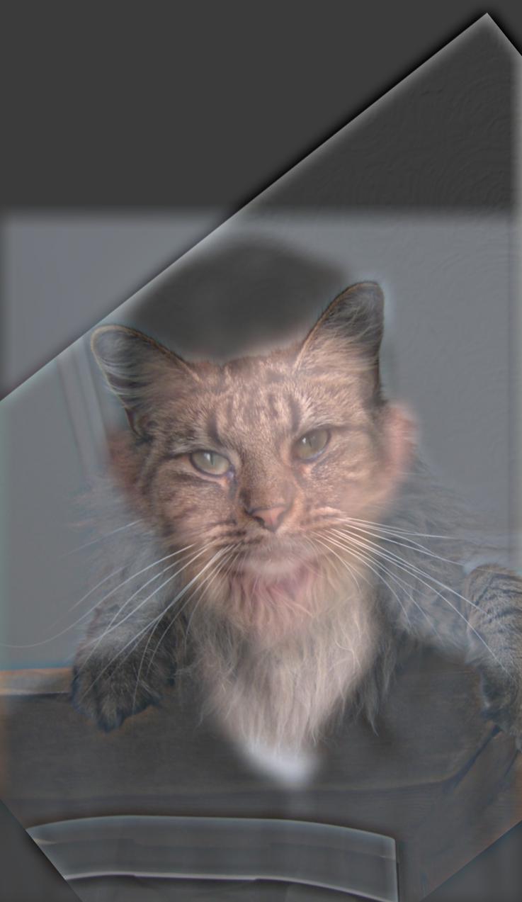
When creating hybrids, it is important that the two images align well. Otherwise, the magical hybrid effect will not work.
I received a special request to combine an "amogus enthusiast", named Jason, with an "amogus drip crewmate".
Unfortunately, because the two subjects did not align well, the hybrid effect was unsuccessful.
Below is the failed case of the "amogus" hybrid:
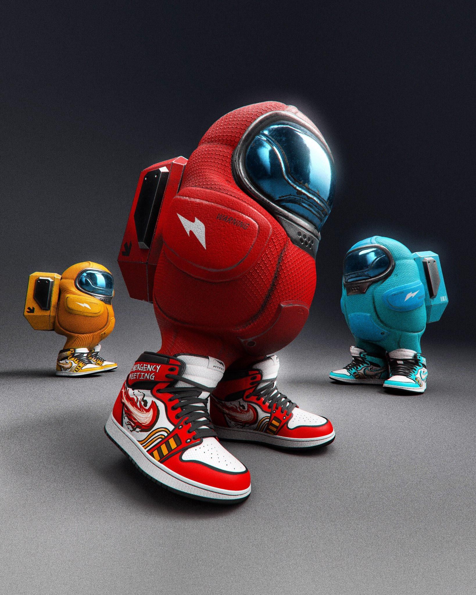
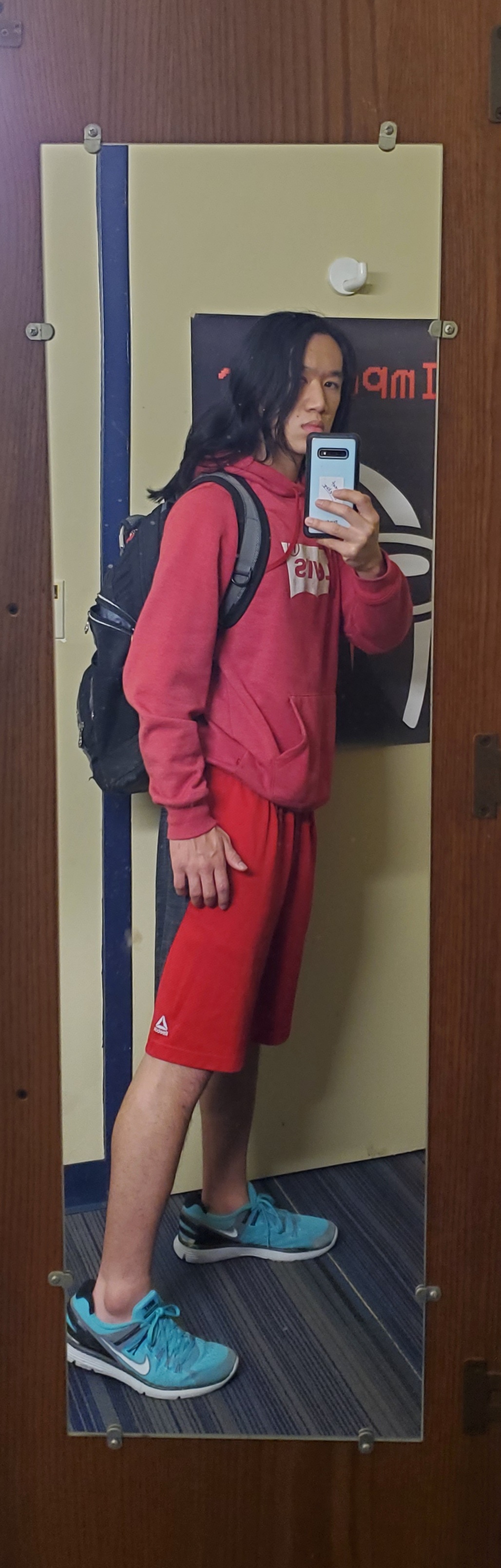
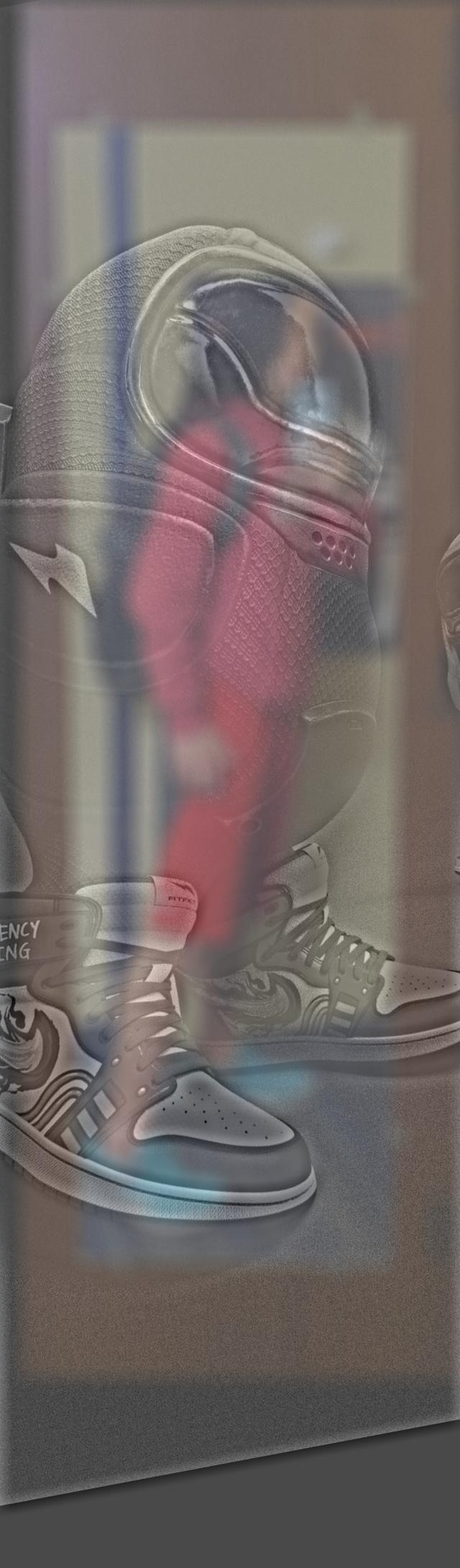
Image Credit: Jason
The following are several successful hybrids:
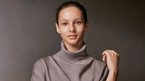
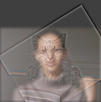
The cat-human hybrid was inspired by the cinematic sensation, Cats (2019). I used Nutmeg's photo for the high frequencies and an image of Francesca Hayward, the main character of Cats, for the low frequencies. Both grayscale and color versions are shown below.
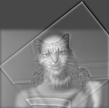
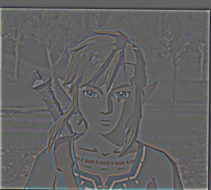
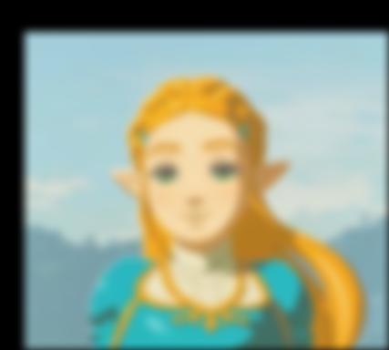
I also made a hybrid of Link and Zelda from the Legend of Zelda franchise. This combination turned out to be the most successful hybrid.
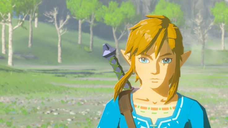
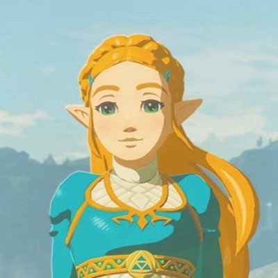
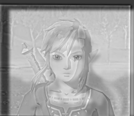
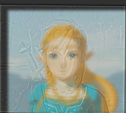
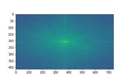
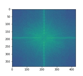
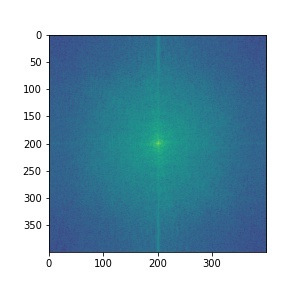
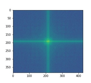
Below illustrates the process of creating the hybrid along with the Fourier analysis images.

The goal is to blend two images seamlessly using multi-resolution blending. This method computes a smooth seam between the images at each level of frequencies. The result is a smoothly blended image.
Before we blend images, we need to implement Gaussian and Laplacian stacks.
In a Gaussian stack, we take an input image and increasingly blur it (convolve it with a Gaussian) at each level. Going down the stack, the image becomes more and more blurred.
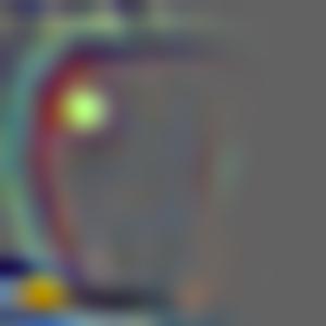
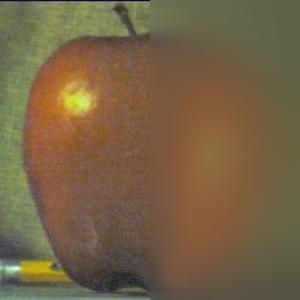
In a Laplacian stack, we take the output images of the Gaussian stack and compute the differences between successive images. For instance, the first image of the Laplacian stack would be computed by taking the first image of the Gaussian stack and subtracting the second image of the Guassian stack. After computing all the difference images, we add the last Gaussian stack image to the Laplacian stack. This way, we will be able to reconstruct the original image by adding together all the images of the Laplacian stack.
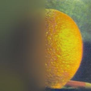
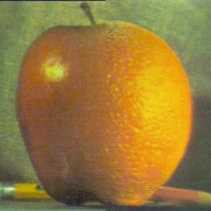
Now, we can use the Gaussian and Laplacian stacks to blend images. In addition to the two images we would like to blend, we also need a black-and-white mask to identify which portions of the images to blend.
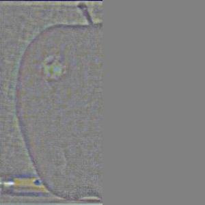
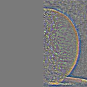
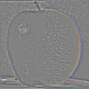
Below is a blend of an apple and an orange, aka the Oraple, with 6 levels.
This blending method can also be used to recreate fictional characters.
Below are two blends inspired from the wildly-popular manga and anime, Jujutsu Kaisen, both using 5 levels.

Image Credit: Jujutsu Kaisen
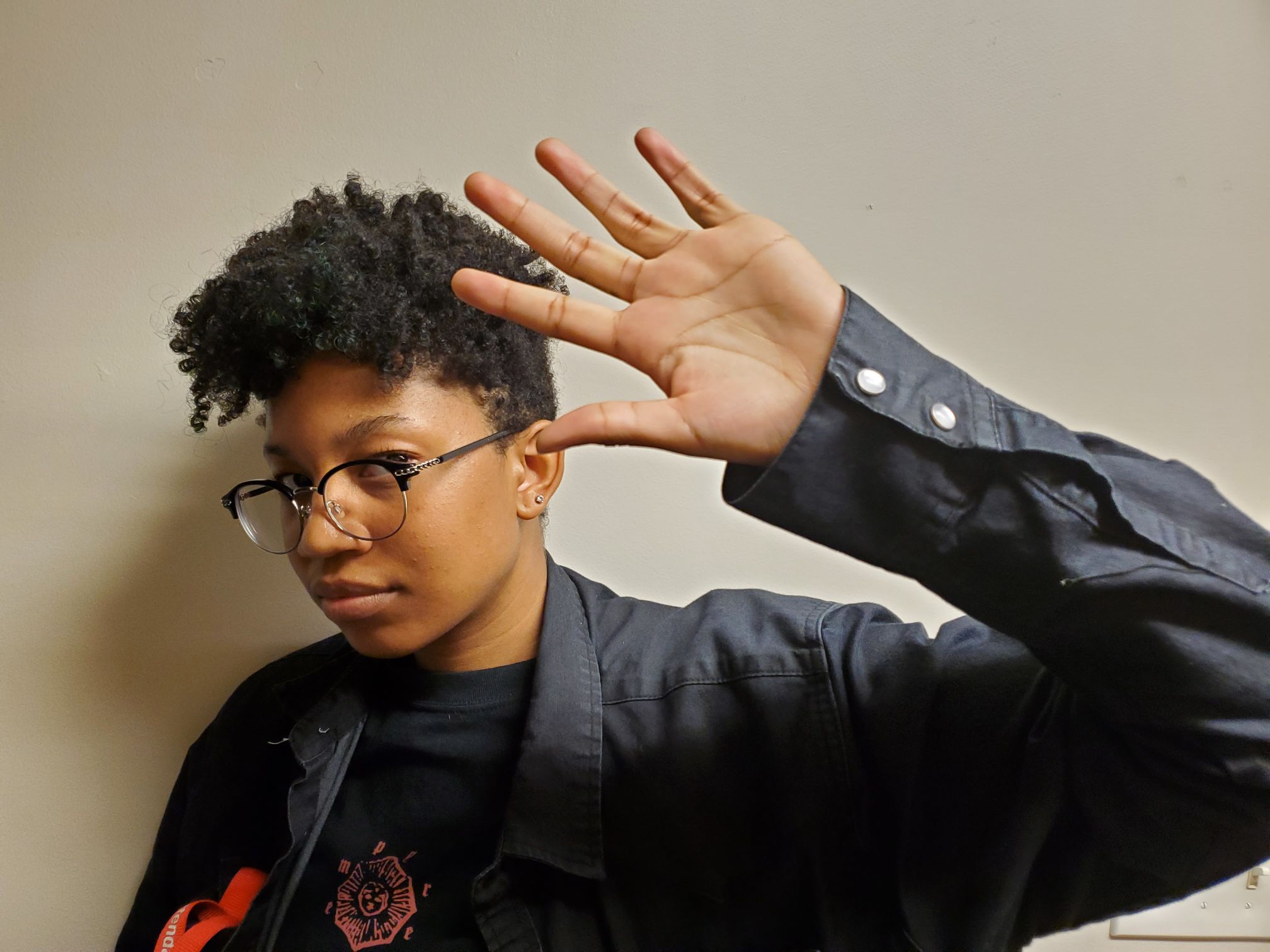
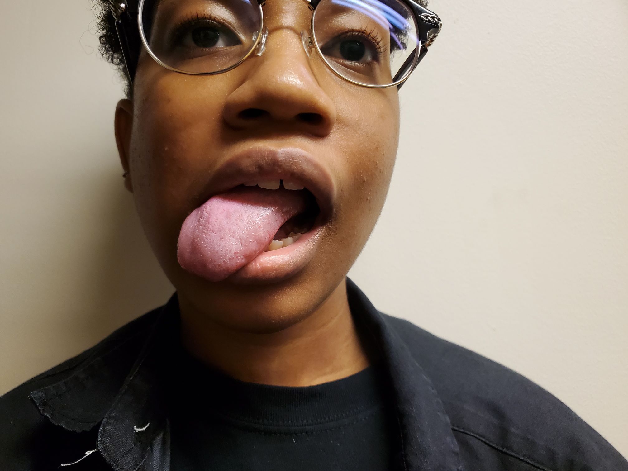
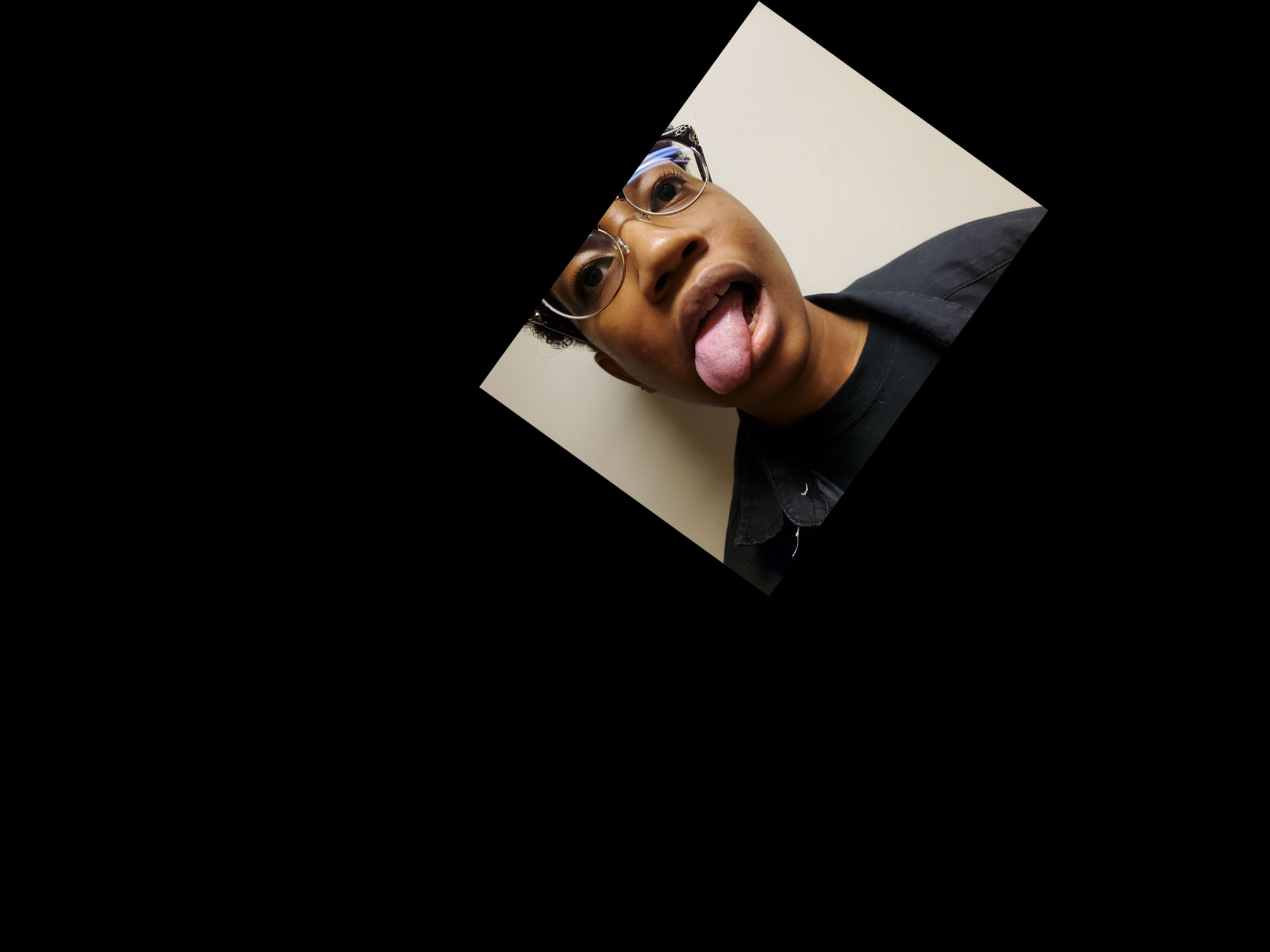
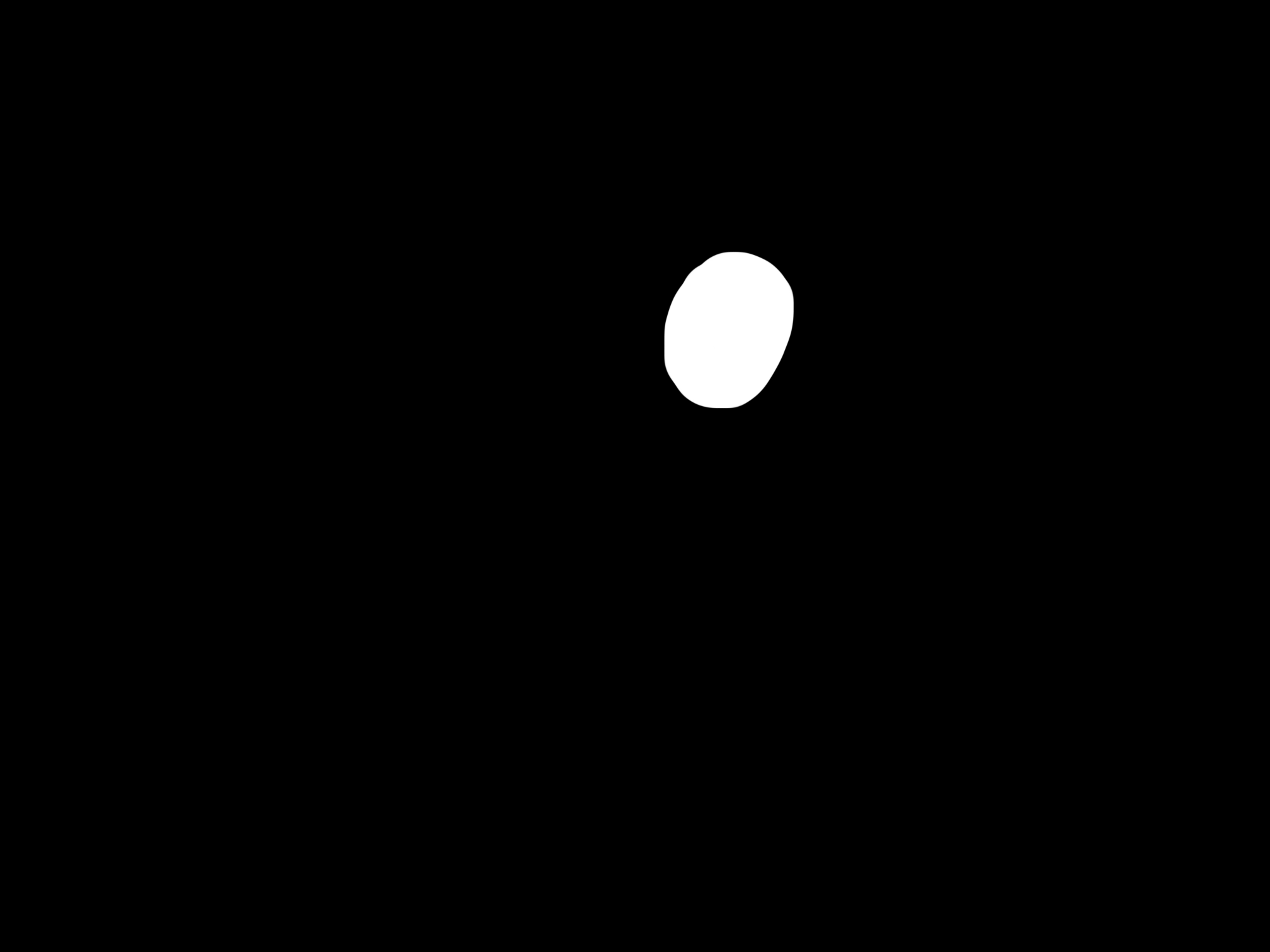
Image Credit: Arren
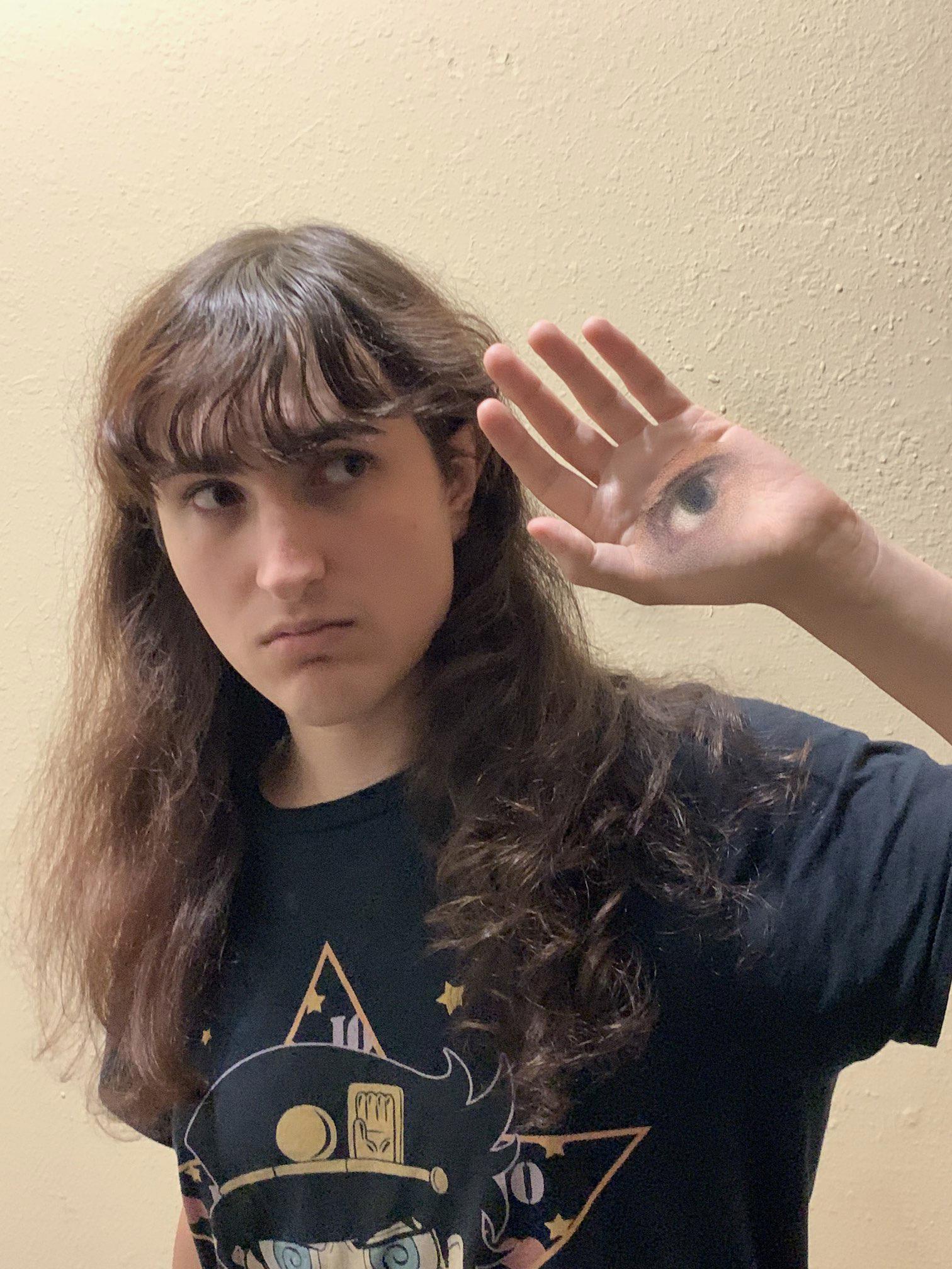
Image Credit: Ivy