Overview

In this project, the goal was to understand how filters and frequencies play a role in computational imaging.

Part 1: Fun with Filters

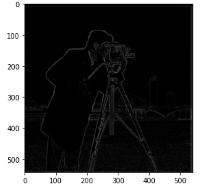
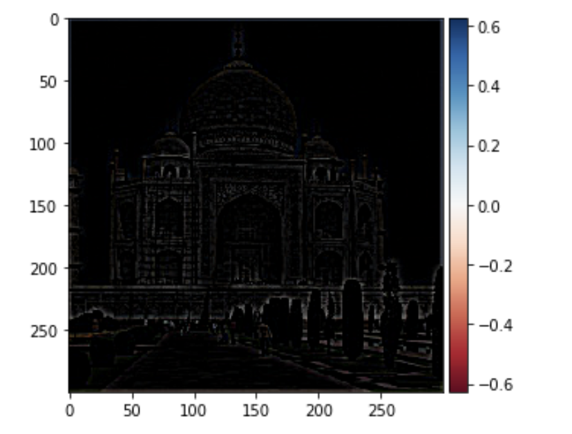
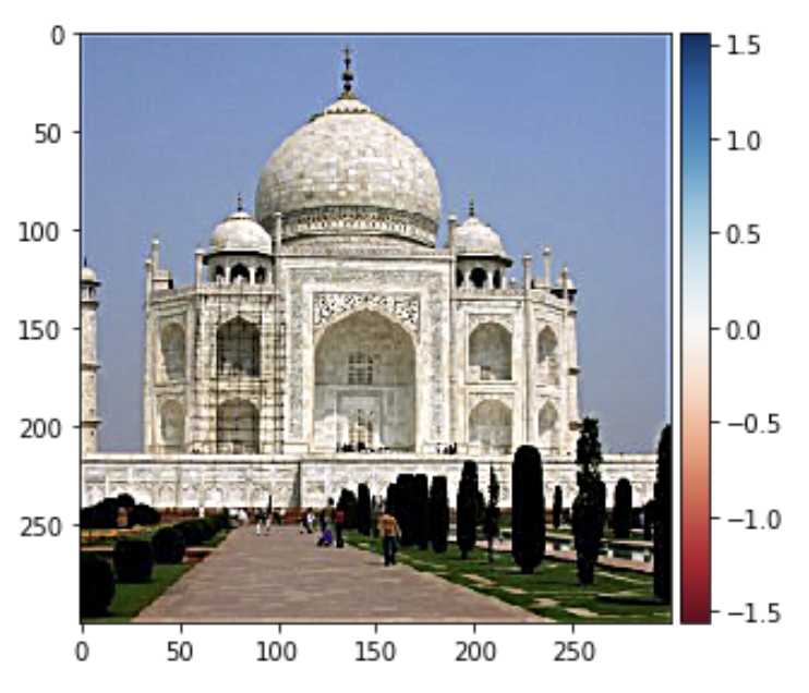
Part 1.1: Gradient Magnitude Approach

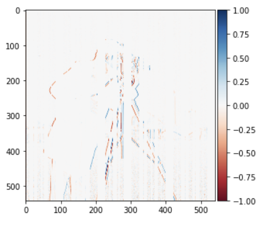
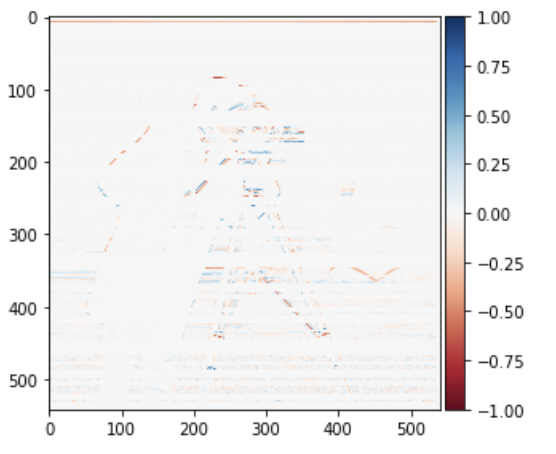
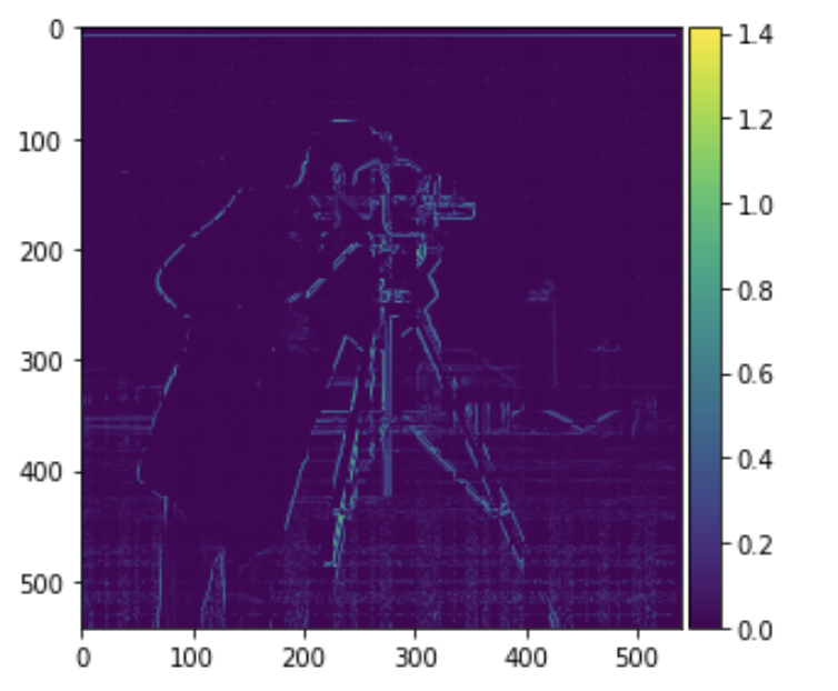
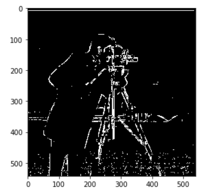
To produce the gradient magnitude image, I first computed the partial derivative images in the x and y directions. Then I ran np.sqrt((grad_x**2) + (grad_y**2)) on the result to obtain the gradient magnitude image.

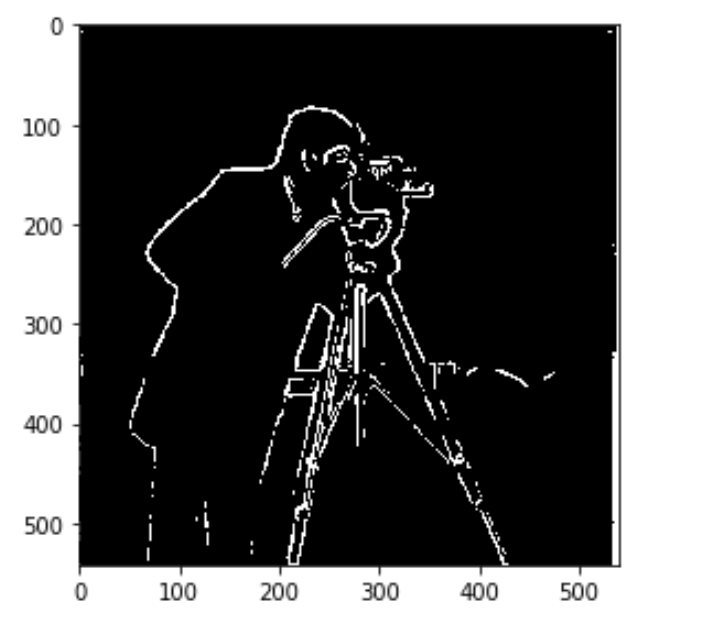
Part 1.2: Derivative of Gaussian Filter

The difference is that the the gaussian filter produces a smoother result than the difference operator as the gaussian filter kills the nosier high frequencies.

Part 2: Fun with Frequencies

Part 2.1: Image Sharpening

Progression to sharp image.

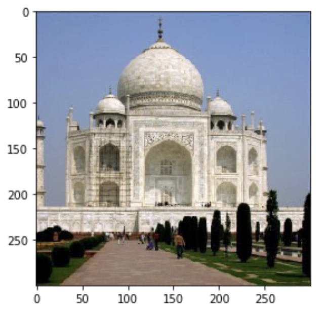
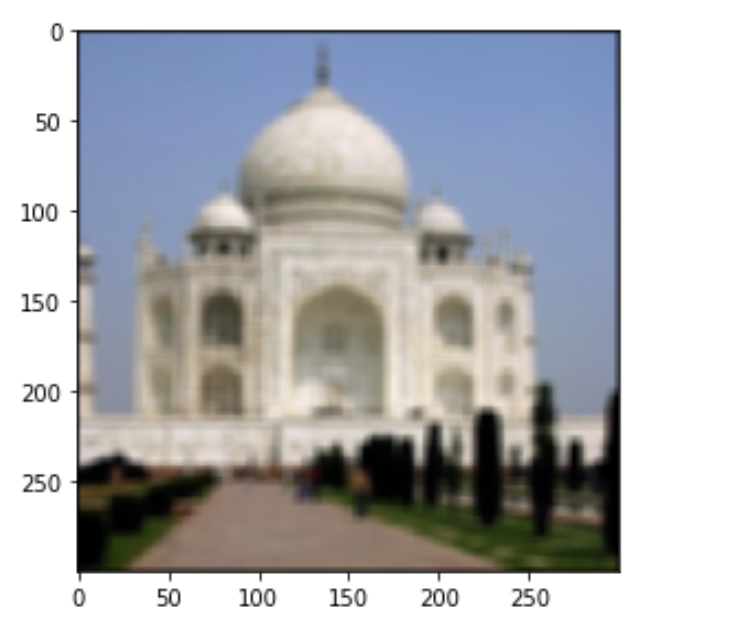
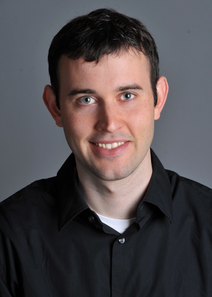
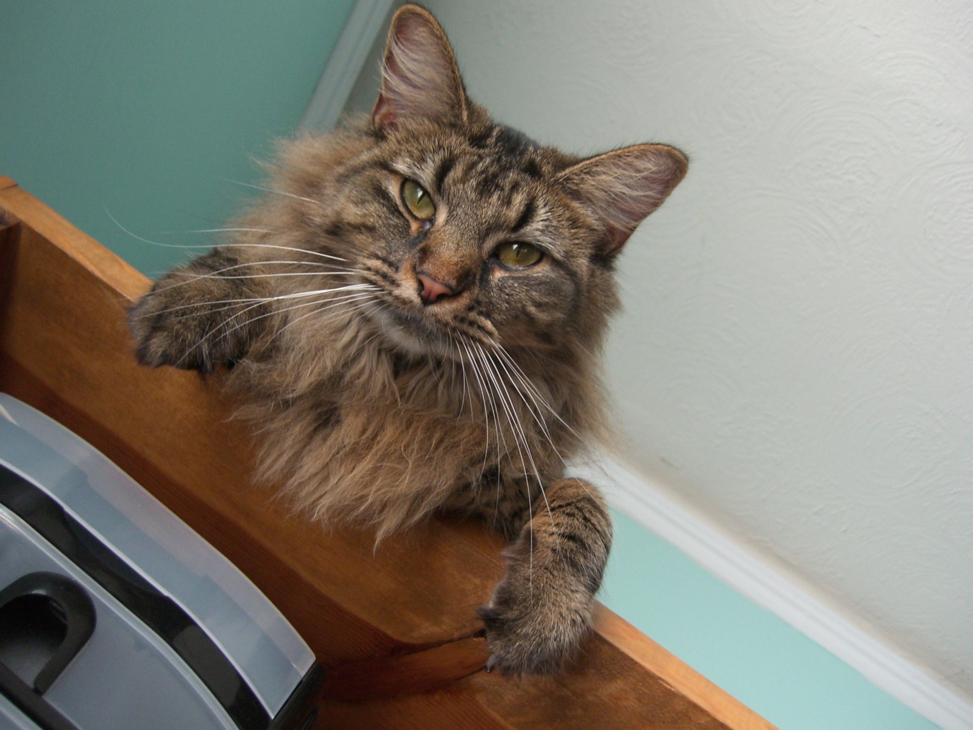
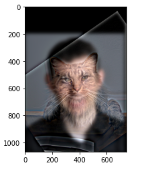
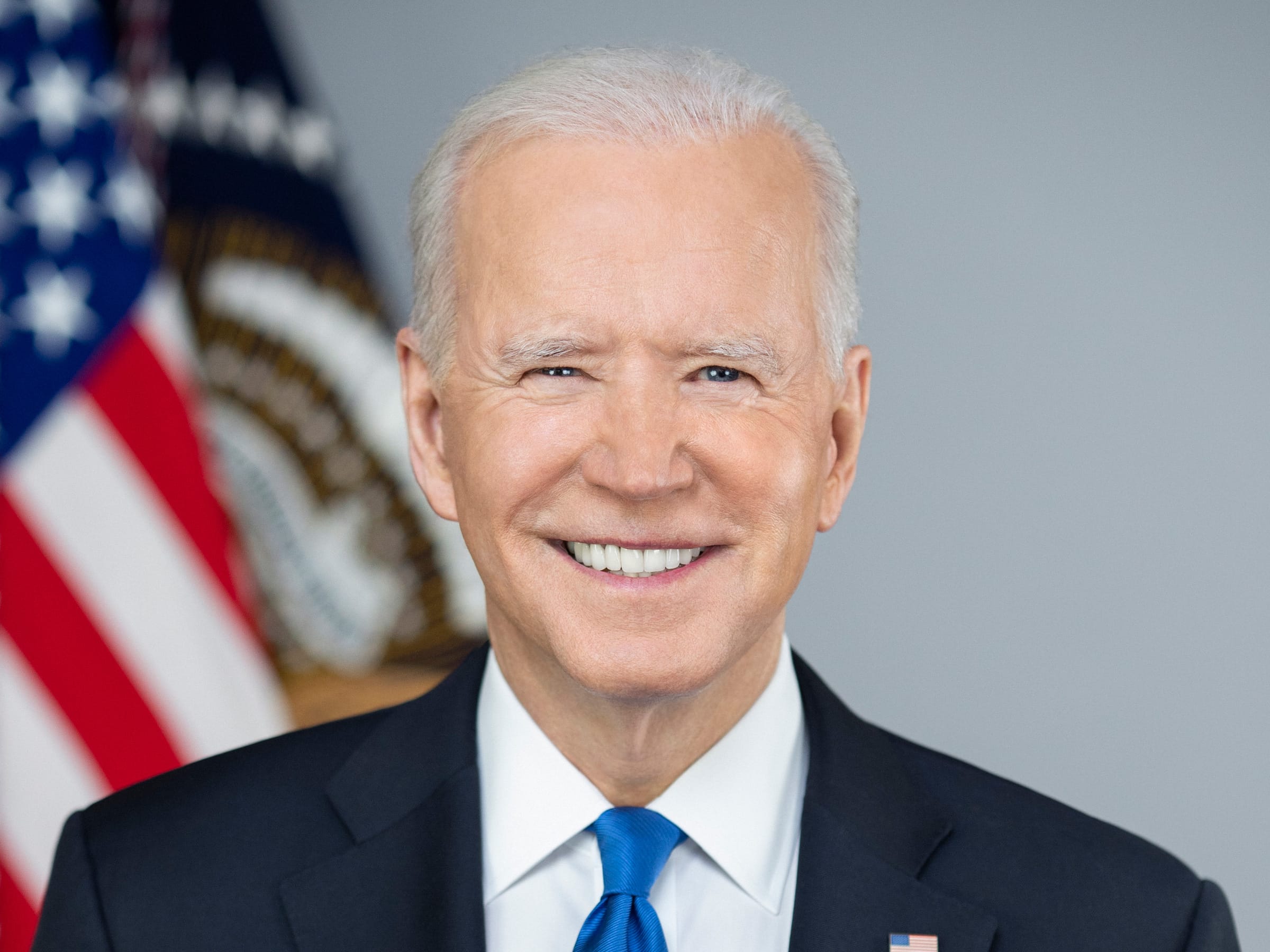
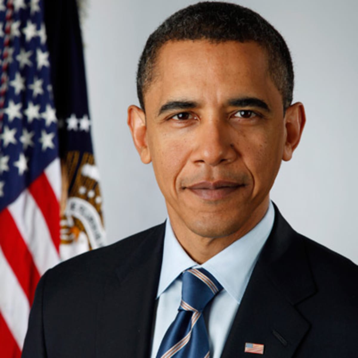
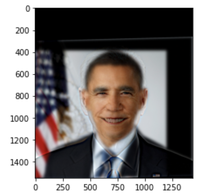
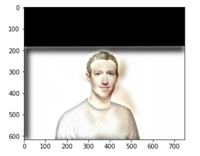
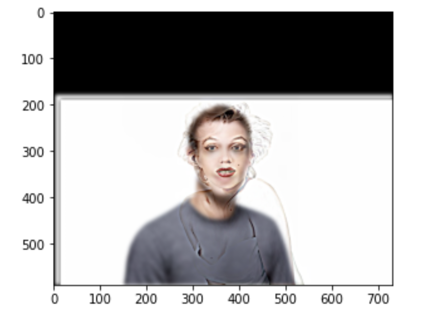
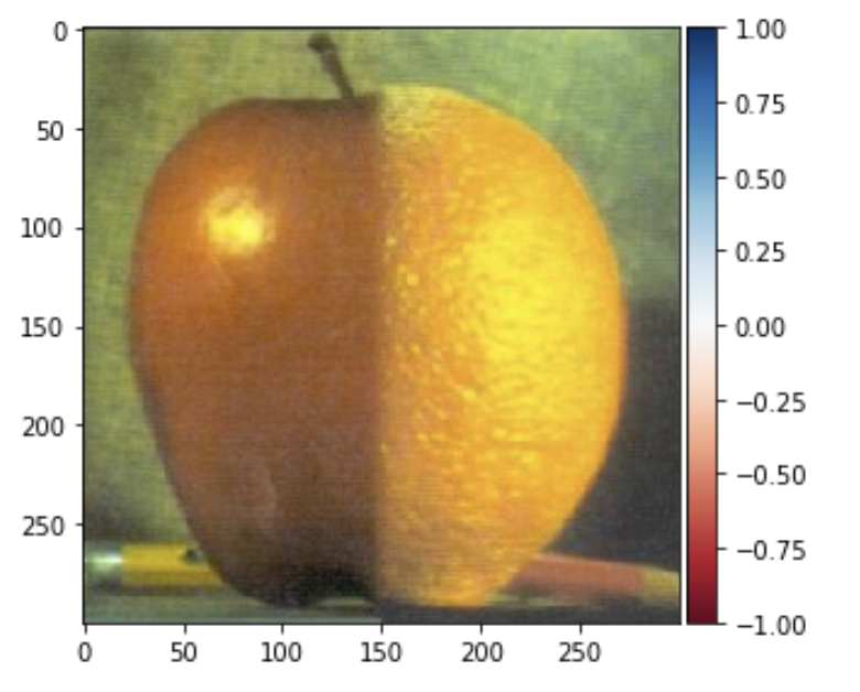
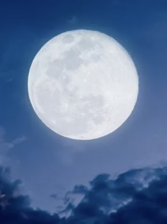
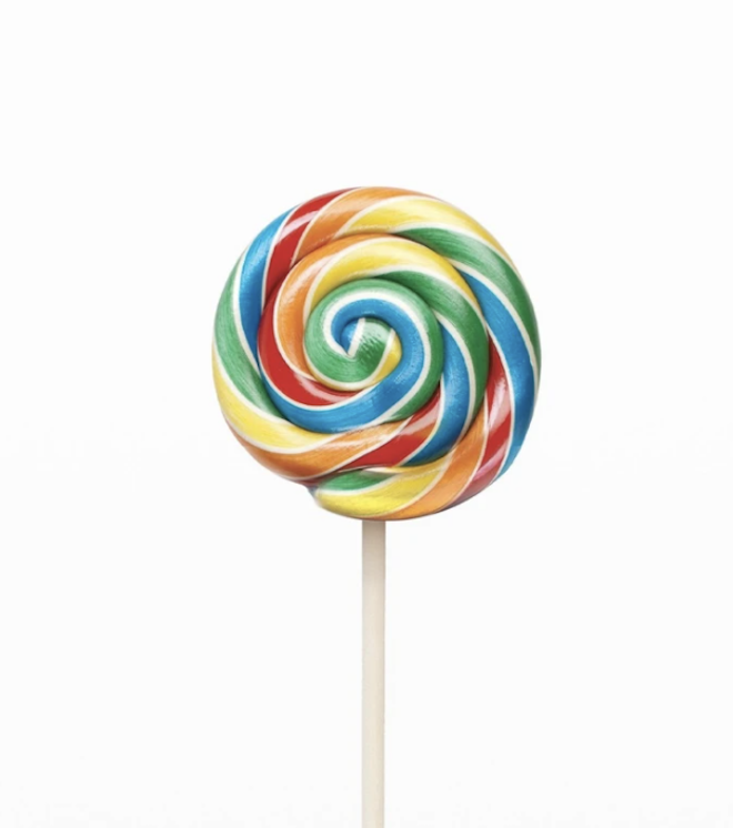
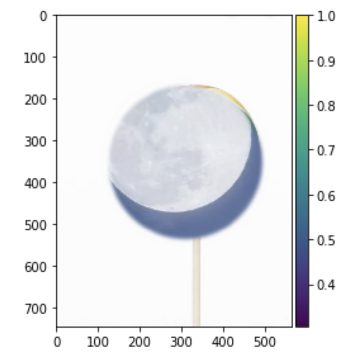
Part 2.2: Hybrid Images

Hybrid Images

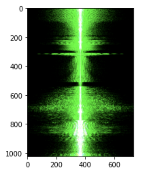
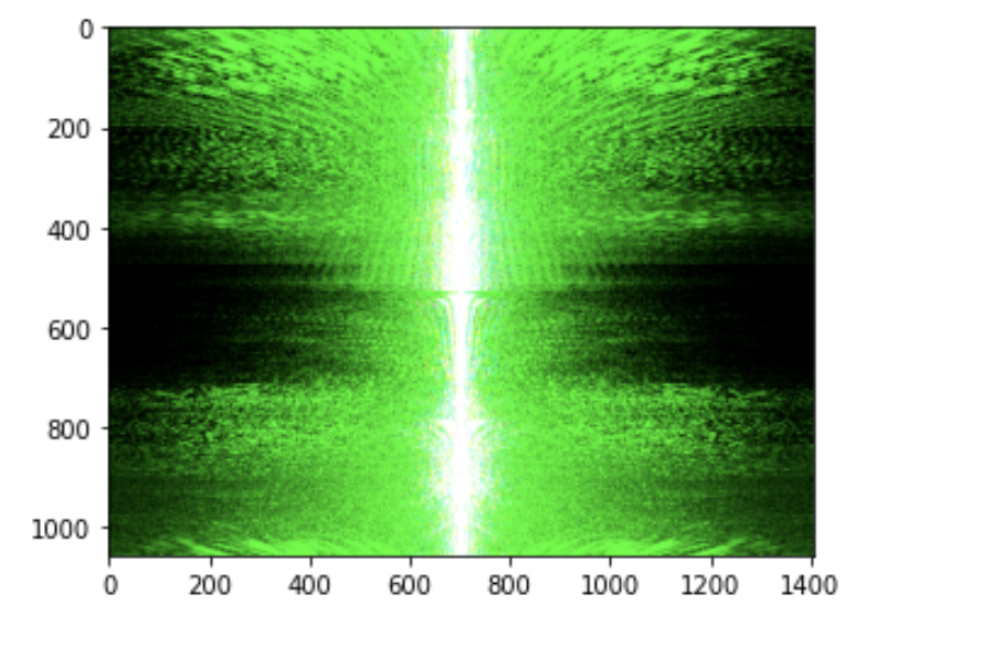
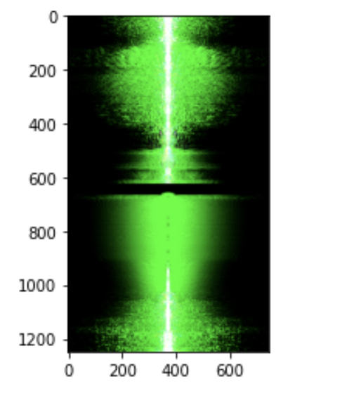
Log Magnitude of Fourier transforms of each respective image.

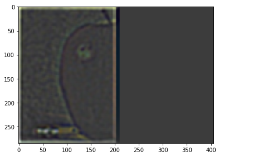
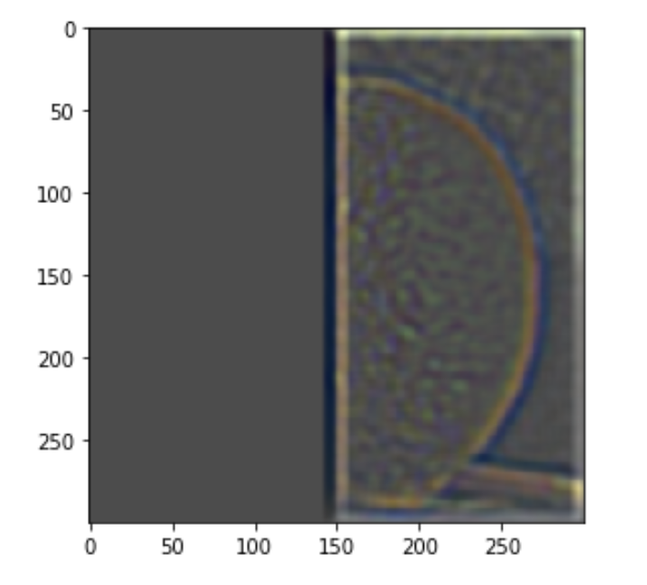
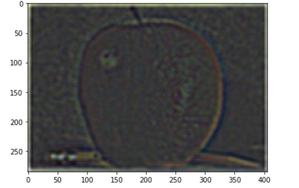
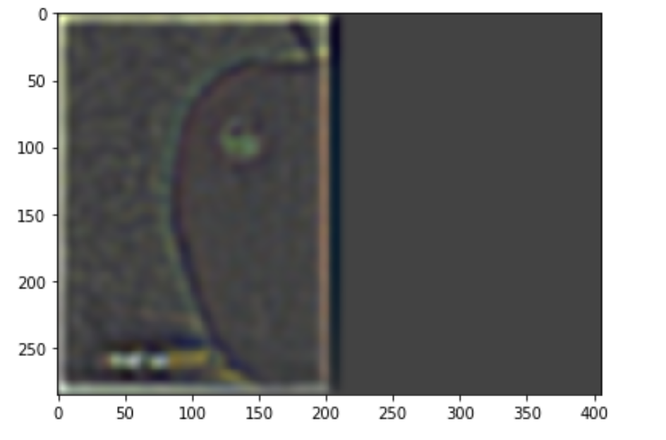
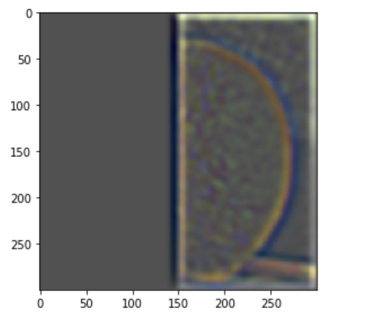
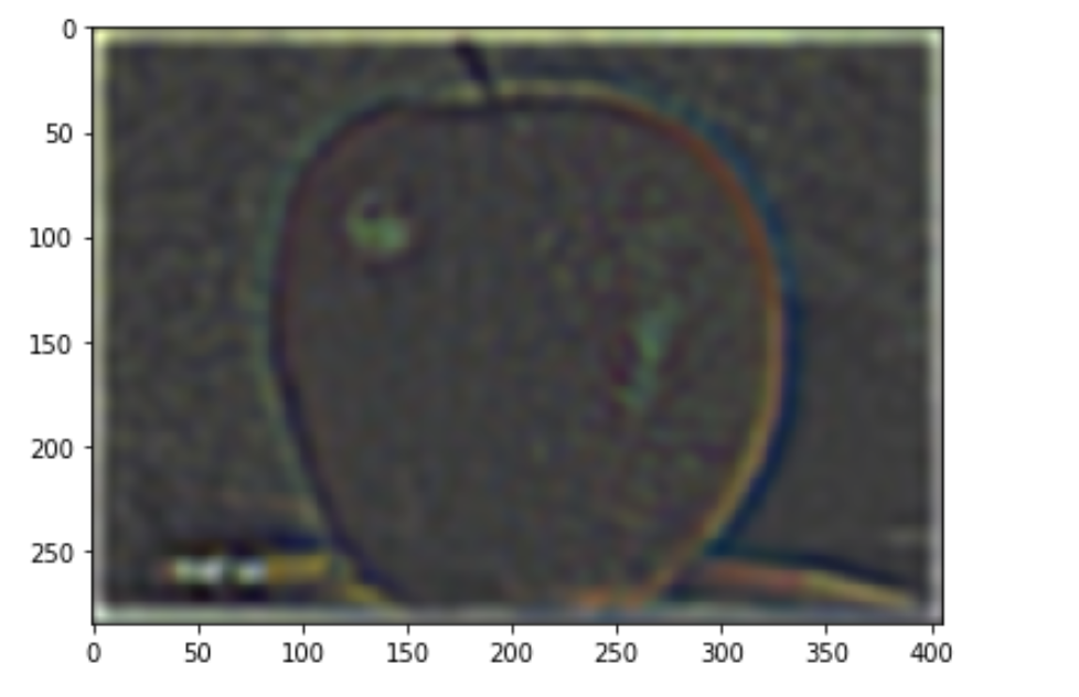
Part 2.3: Gaussian and Laplacian Stacks

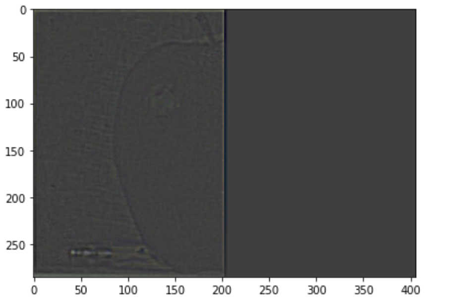
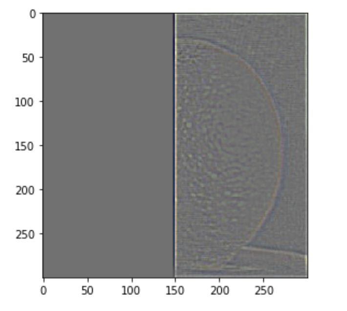
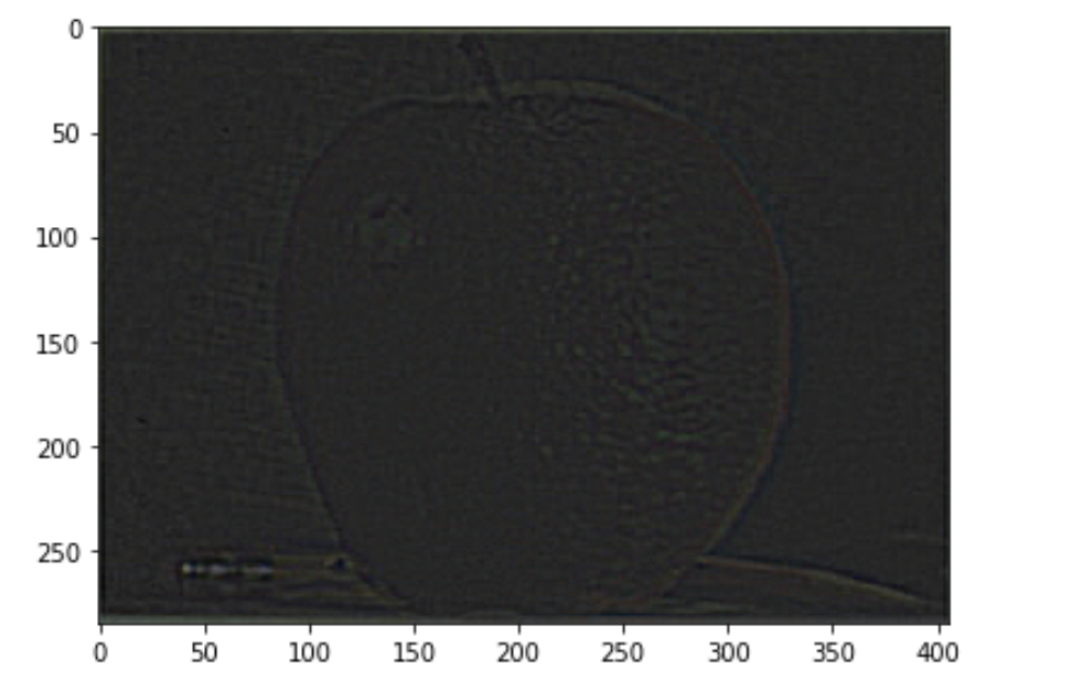
Above: Laplacian pyramid blending details as in Burt and Adelson 1983b. First three rows show the high, medium, and low frequency parts of the laplacian pyramid from levels 0, 2, and 4.

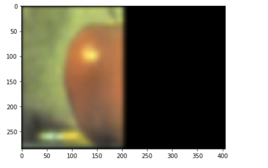
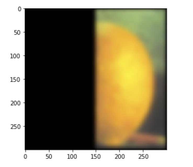
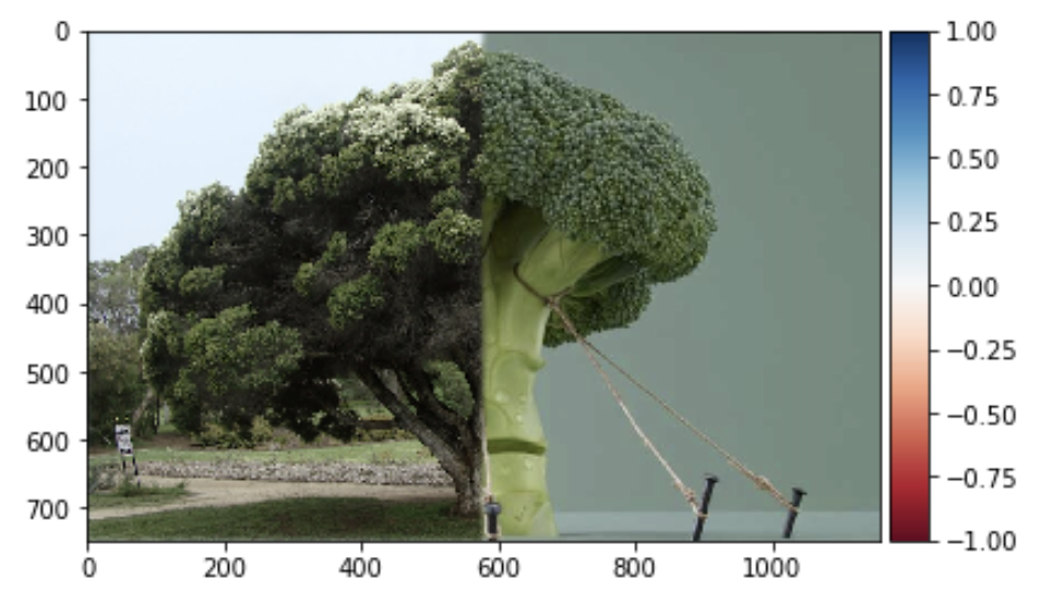
Part 2.4: Multi-resolution Blending

More blending

Even more blending (irregular mask)

The most important learning

The most important learning from this project is filtering out high frequency noise with gaussian filters to obtain smoother and better-looking image outputs.