

The derivative images \(d_x\) and \(d_y\) is computed with the filters \(D_x=\begin{bmatrix}1 & -1\end{bmatrix}\) and \(D_y=\begin{bmatrix}1\\-1\end{bmatrix}\) respectively.
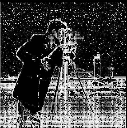
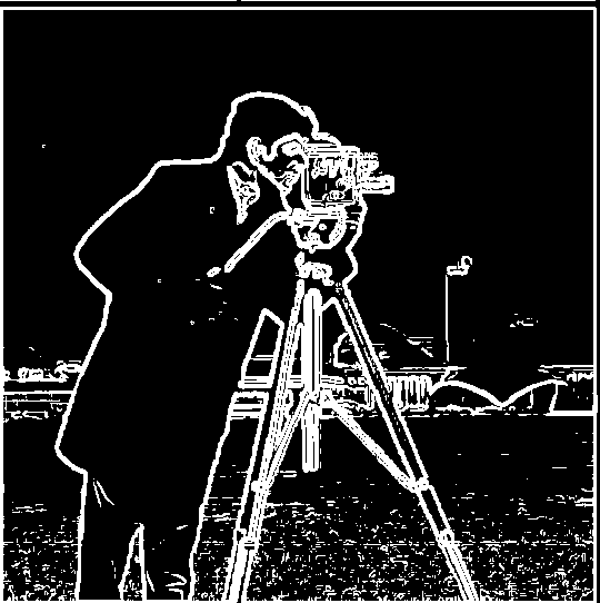
The magnitude image is computed as: \(magnitude = \sqrt{d_x^2+d_y^2}\).

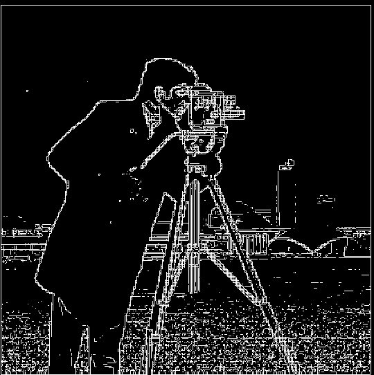
Images generated with different threshold values are shown below.
 Threshold=0.00 |
 Threshold=0.01 |
 Threshold=0.02 |
 Threshold=0.03 |
 Threshold=0.04 |
 Threshold=0.05 |
 Threshold=0.06 |
 Threshold=0.07 |
 Threshold=0.08 |
 Threshold=0.09 |
 Threshold=0.10 |
 Threshold=0.11 |
 Threshold=0.12 |
 Threshold=0.13 |
 Threshold=0.14 |
 Threshold=0.15 |
 Threshold=0.16 |
 Threshold=0.17 |
 Threshold=0.18 |
 Threshold=0.19 |
 Threshold=0.20 |
 Threshold=0.21 |
 Threshold=0.22 |
 Threshold=0.23 |
 Threshold=0.24 |
 Threshold=0.25 |
 Threshold=0.26 |
 Threshold=0.27 |
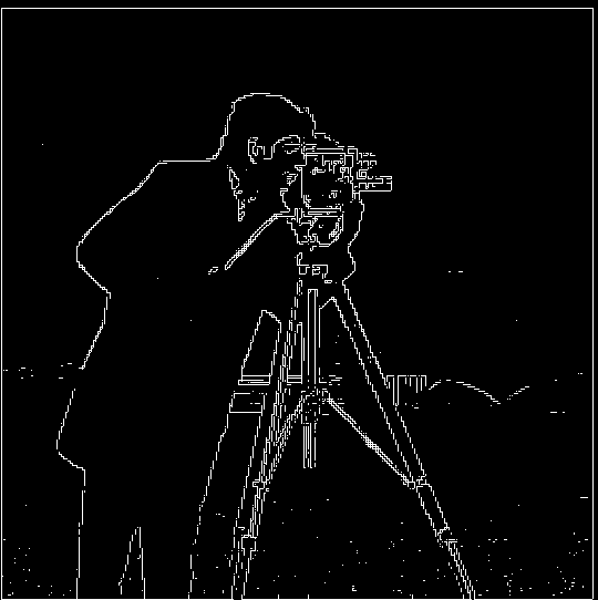
In my opinion, \(threshold=0.26\) is the best in terms of filtering out the noise, as shown below.
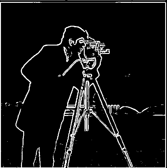
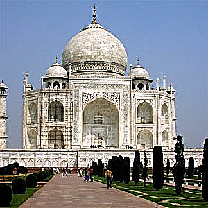
The filter half-width is recommended to be about \(3\sigma\), so I applied \(7\times 7\) Gaussian kernel with \(\sigma=1.0\) to the target image as shown below.


The derivative images \(d_x\) and \(d_y\) are shown below.


The magnitude image is shown below with the one from Part 1.1.

Images generated with different threshold is shown below.
 Threshold=0.00 (Gaussian) |
 Threshold=0.01 (Gaussian) |
 Threshold=0.02 (Gaussian) |
 Threshold=0.03 (Gaussian) |
 Threshold=0.04 (Gaussian) |
 Threshold=0.05 (Gaussian) |
 Threshold=0.06 (Gaussian) |
 Threshold=0.07 (Gaussian) |
 Threshold=0.08 (Gaussian) |
 Threshold=0.09 (Gaussian) |
 Threshold=0.10 (Gaussian) |
 Threshold=0.11 (Gaussian) |
 Threshold=0.12 (Gaussian) |
 Threshold=0.13 (Gaussian) |
 Threshold=0.14 (Gaussian) |
 Threshold=0.15 (Gaussian) |
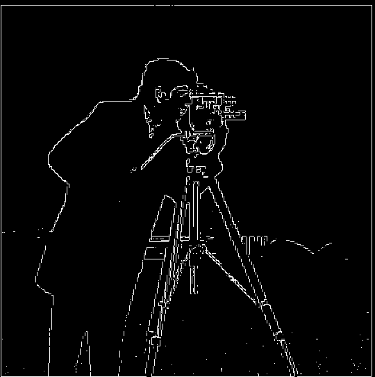
When the Gaussian filter is applied to the original image, the resulting edges become much stronger and more apparent as shown below.
Threshold=0.26 |
Threshold=0.05 (Gaussian) |
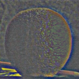
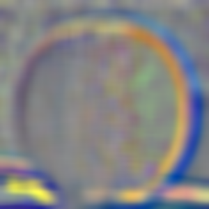
Now we can do the same thing with a single convolution instead of two by creating a derivative of gaussian filters. Convolving a \(7\times 7\) Gaussian filter with D_x and D_y and the resulting DoG filters are shown below.

As a part of sanity check, we are getting the same results with a single-step Gaussian filtering.
Threshold=0.05 (Two-step Gaussian) |
 Threshold=0.05 (Single-step Gaussian) |
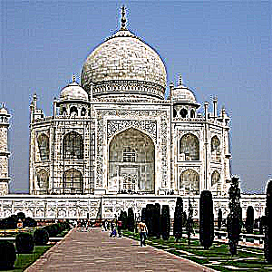
A high-frequency image \(H\) can be computed with the difference between the original image \(X\) and its Gaussian filtered image \(G(X)\); \(H=X-G(X)\).
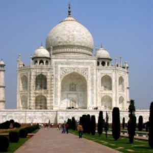
To obtain the sharpened image \(S\), defining the hyperparameter \(\alpha\) to control the level of sharpness, we have the derivation as it follows:
$$ S = X + \alpha H $$
 Original image X |
 Blurred with Gaussian filter G(X) |
 (Original image - blurred image) H |
 Sharpened image (alpha=0.1) |
 Sharpened image (alpha=0.5) |
 Sharpened image (alpha=1.0) |
 Sharpened image (alpha=5.0) |
 Sharpened image (alpha=10.0) |
 Sharpened image (alpha=100.0) |
Other results:
 Original image X |
 Blurred with Gaussian filter G(X) |
 (Original image - blurred image) H |
 Sharpened image (alpha=0.1) |
 Sharpened image (alpha=0.5) |
 Sharpened image (alpha=1.0) |
 Sharpened image (alpha=5.0) |
 Sharpened image (alpha=10.0) |
 Sharpened image (alpha=100.0) |
Close-up view
Original image X |
Sharpened image (alpha=1.0) |
Other results:
 Original image X |
 Blurred with Gaussian filter G(X) |
 (Original image - blurred image) H |
 Sharpened image (alpha=0.1) |
 Sharpened image (alpha=0.5) |
 Sharpened image (alpha=1.0) |
 Sharpened image (alpha=5.0) |
 Sharpened image (alpha=10.0) |
 Sharpened image (alpha=100.0) |
Close-up view
Original image |
Sharpened image (alpha=1.0) |
For a sanity check, instead of adding \(\alpha H\) to the original image, we can add the value to the blurred image G(X) to see if sharpening would bring the original image back. In math, the new sharpend image \(S^*\) is defined as:
$$ S^* = G(X) + \alpha H $$
Original image X |
Blurred with Gaussian filter G(X) |
(Original image - blurred image) H |
 Sharpened image (G(X) + 0.1 H) |
 Sharpened image (G(X) + 0.5 H) |
 Sharpened image (G(X) + 1.0 H) |
 Sharpened image (G(X) + 5.0 H) |
 Sharpened image (G(X) + 10.0 H) |
 Sharpened image (G(X) + 100.0 H) |
As easily predicted, when \(\alpha = 1.0\), the sharpend image becomes the same as the original image (\(X=G(X)+H=G(X)+(X-G(X))\)).
The gaussian filter with \(\sigma\) as its standard deviation in the spacial domain is known to follow the same Gaussian distribution in the frequency domain but with \(\frac{1}{\sigma}\) as its new standard deviation.
As Figure 5 in the Hybrid images paper illustrated, the gap between two frequency curves for low- and high- spacial frequencies at \(Gain=0.5\) is considered to be a better hybrid image, we should try to make the low-spacial scale have a smaller standard deviation and make the high-spacial scale have a larger standard deviation both in the frequency domain. This implies that we are recommended to use a large \(\sigma\) for our low-pass filter and a small \(sigma\) for our high-pass filter in a spacial domain.
Hence, for this experiment, I set \(\sigma=11\) for low-pass Gaussian filter and \(\sigma=4\) for high-pass Gaussian filter.
 Rotated Original image A |
 Rotated Original image B |
 Low-pass filtered A with \(\sigma=11\) |
 High-pass filtered B with \(\sigma=4\) |
 Low-pass A + High-pass B |
 Rotated Original image A (Fourier) |
 Rotated Original image B (Fourier) |
 Low-pass filtered A with \(\sigma=11\) (Fourier) |
 High-pass filtered B with \(\sigma=4\) (Fourier) |
 Low-pass A + High-pass B (Fourier) |
Other images: Normal + Grinning Aphex Twin
 Rotated Original image A |
 Rotated Original image B |
 Low-pass filtered A with \(\sigma=4\) |
 High-pass filtered B with \(\sigma=3\) |
 Low-pass A + High-pass B |
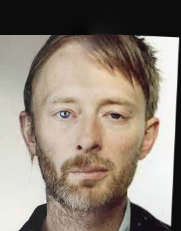
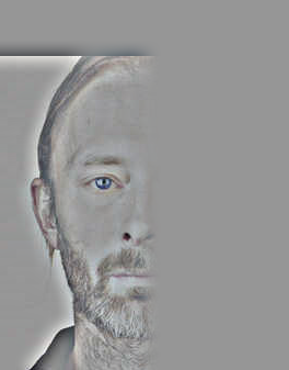
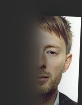
Other images: Young + Old Tom Yorke from Radiohead
 Rotated Original image A |
 Rotated Original image B |
 Low-pass filtered A with \(\sigma=4\) |
 High-pass filtered B with \(\sigma=3\) |
 Low-pass A + High-pass B |
 Gaussian stacks (apple) - Level 1 |
 Gaussian stacks (apple) - Level 2 |
 Gaussian stacks (apple) - Level 3 |
 Gaussian stacks (apple) - Level 4 |
 Gaussian stacks (apple) - Level 5 |
 Laplacian stacks (apple) - Level 1 |
 Laplacian stacks (apple) - Level 2 |
 Laplacian stacks (apple) - Level 3 |
 Laplacian stacks (apple) - Level 4 |
 Laplacian stacks (apple) - Level 5 |
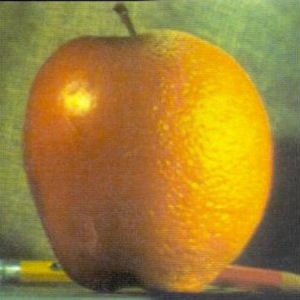
 Gaussian stacks (orange) - Level 1 |
 Gaussian stacks (orange) - Level 2 |
 Gaussian stacks (orange) - Level 3 |
 Gaussian stacks (orange) - Level 4 |
 Gaussian stacks (orange) - Level 5 |
 Laplacian stacks (orange) - Level 1 |
 Laplacian stacks (orange) - Level 2 |
 Laplacian stacks (orange) - Level 3 |
 Laplacian stacks (orange) - Level 4 |
 Laplacian stacks (orange) - Level 5 |
Recreating Figure 3.42 in Szelski (Ed 2) page 167:
 (a) |
 (b) |
 (c) |
 (d) |
 (e) |
 (f) |
 (g) |
 (h) |
 (i) |
 (j) |
 (k) |
 (l) |
Other images: Noon + Afternoon lake (Tazawa lake in Akita, Japan)
 Original image A |
 Original image B |
 Original filter image |
 Result image |
Other images: Tokyo Tower + Fireworks
 Original image A |
 Original image B |
 Original filter image |
 Result image |
Other images: Young + Old Tom Yorke
 Original image A |
 Original image B |
 Original filter image |
 Result image |
Recreating Figure 3.42 in Szelski (Ed 2) page 167:
 (a) |
 (b) |
 (c) |
 (d) |
 (e) |
 (f) |
 (g) |
 (h) |
 (i) |
 (j) |
 (k) |
 (l) |