Part 1.1: Finite Difference Operator
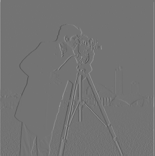
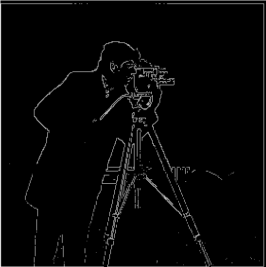
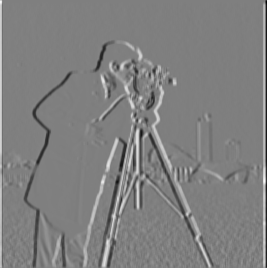
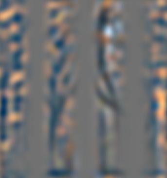
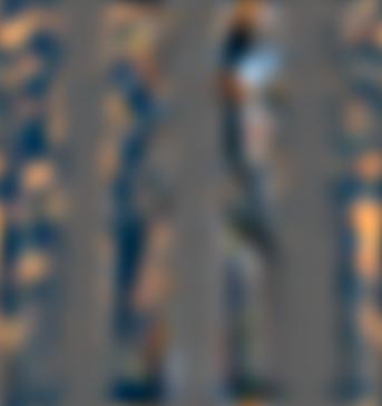
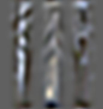
To compute the gradient, first I computed the partial derivatives of the image. For the derivative with respect to x, I convolved the image with [-1, 1]. For the derivate with respect to y, I convolved the image with [[-1], [1]]. This gave the horizontal edges below. I then computed the gradient magnitude with the following computation:
$$\sqrt{(\frac{\partial f}{\partial x})^2 + (\frac{\partial f}{\partial y})^2}$$
Part 1.2: Derivative of Gaussian (DoG) Filter
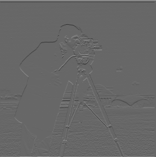
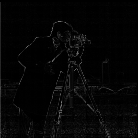
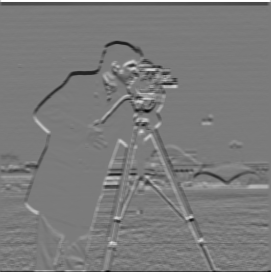
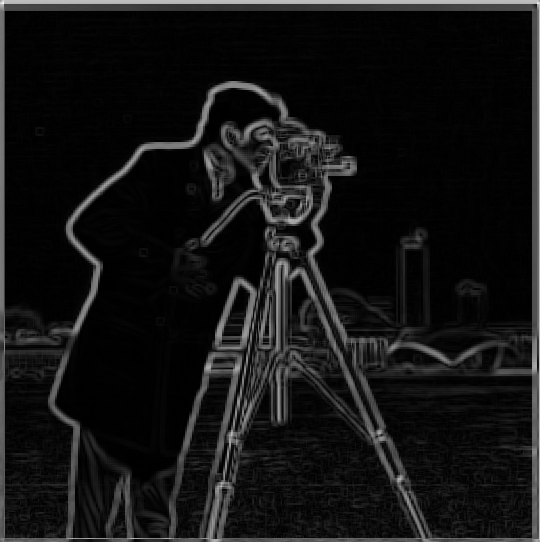
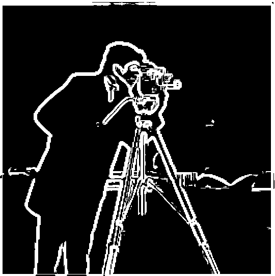
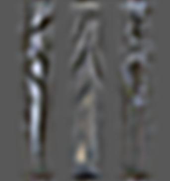
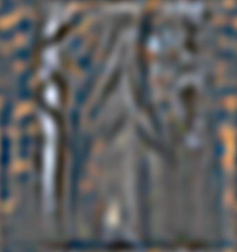
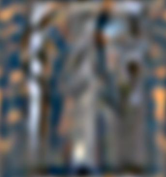
The images below were created using the Gaussian filter as well as the derivative. To get the filter, I found the derivative of the Gaussian filter by convolving the Gaussian with the vectors mentioned in part 1.1.
Comparing it to the results without the Gaussian, we can immediately see that in the partial derivatives of the blurred image the edges are more prominent than without the Gaussian filter. As a result, the gradient magnitude is also better defined, as it is able to capture more details (such as the creases in the pants) without much noise.
Part 2.1: Image Sharpening
For unsharp masking, I first blurred the images using a Gaussian filter. Next, I extracted the high frequencies of the image by computing the difference of the original image and the filtered image. Lastly, I sharpened the image by adding more of the high frequencies into the image and clipping the values outside of [0, 1].
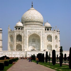 Original image
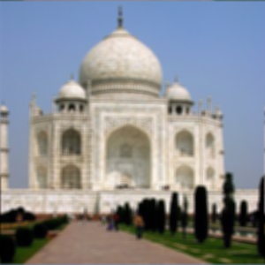
Filtered image
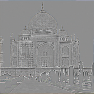
High frequencies
Original image - filtered image

Sharpened image
Original image + high frequencies
 Original image
Filtered image
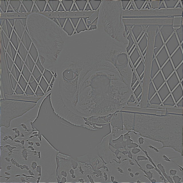
High frequencies
Original image - filtered image
Sharpened image
Original image + high frequencies
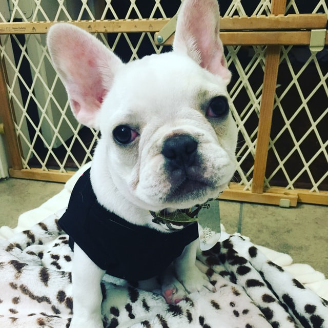
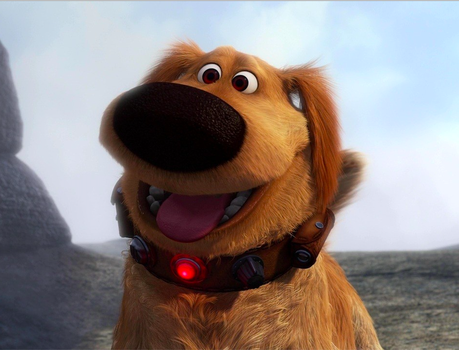
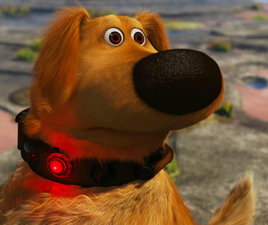
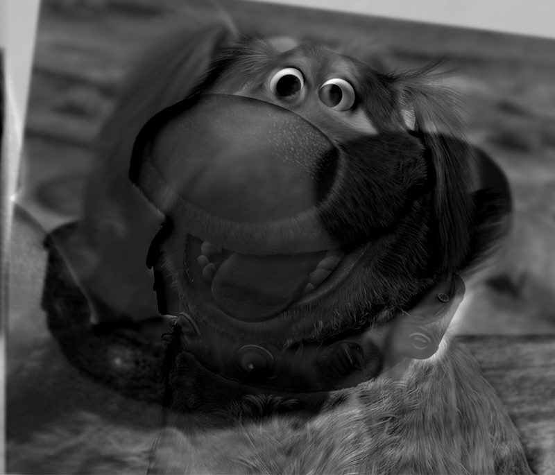
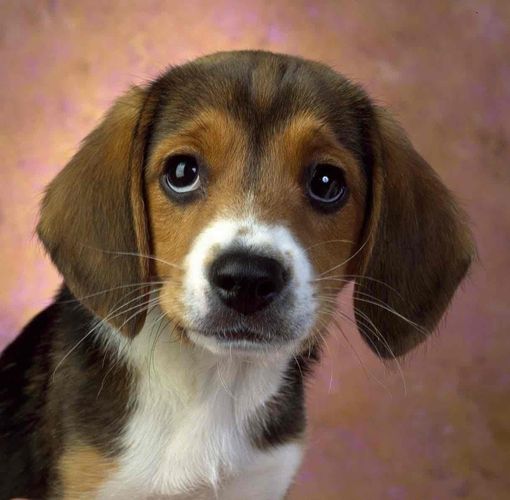
I also tested what would happen if I sharpened an image that was already blurry. I first created a blurry image of the dog (middle photo below) and then applied unsharp masking on that blurry image to get the outcome on the right. It still does not look exactly like the original image, but has more structure than the blurry version such as more definition around the head and fence behind. Some of the less prominent edges such as on the face or body are still not as sharp as the original image.
Original image
Original (blurry) image 
Sharpened image
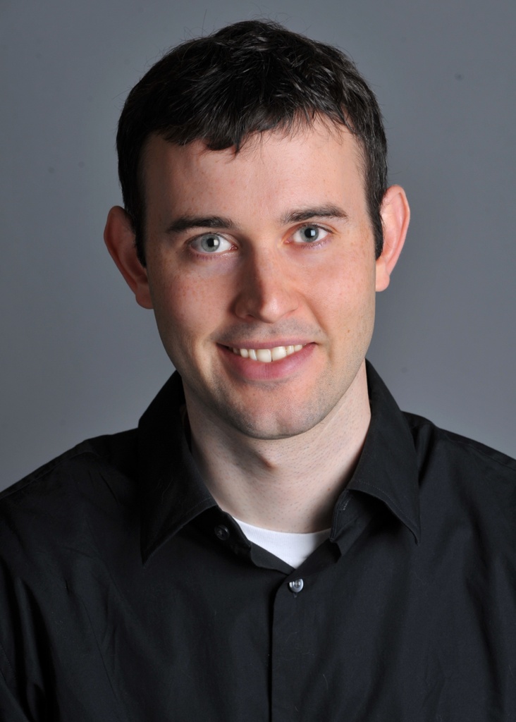
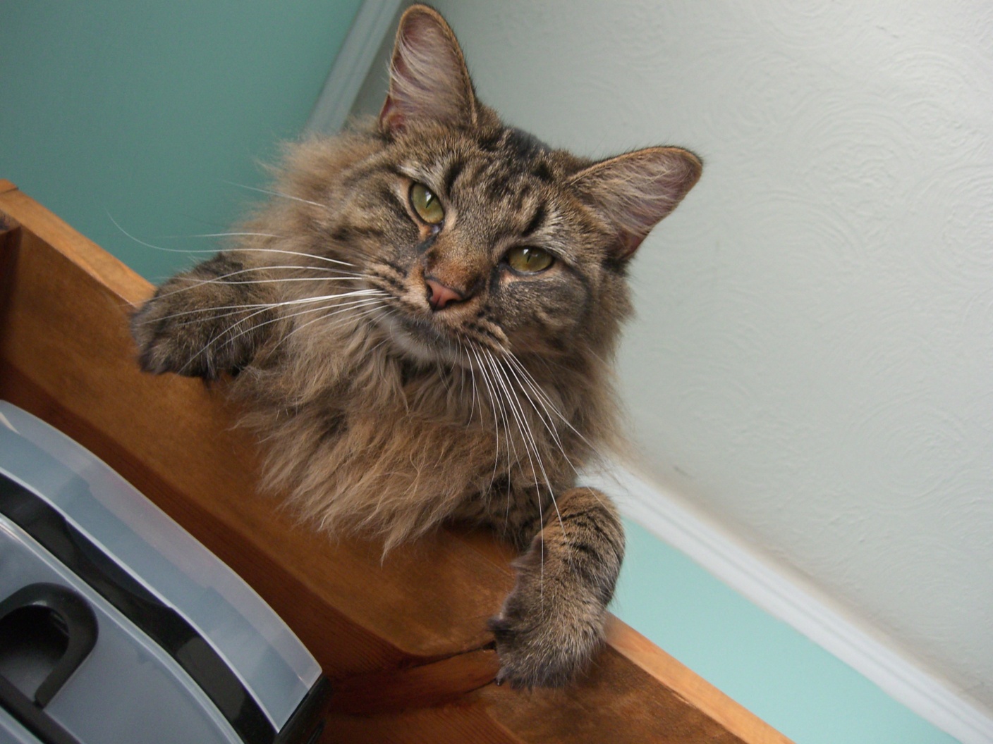
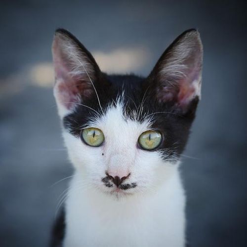
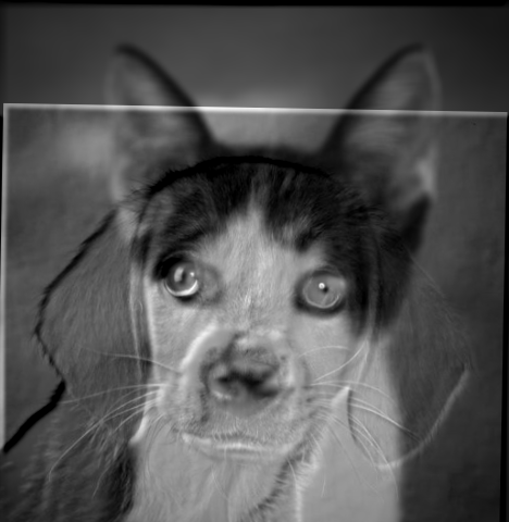
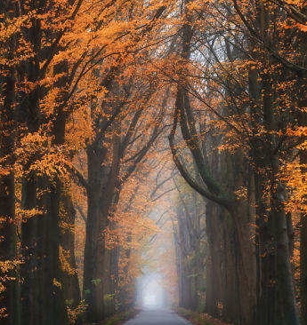
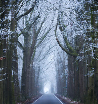
Part 2.2: Hybrid Images
For hybrid images I generated the low frequencies of the one image and the high frequencies of another after aligning them. I then averaged them together to produce the hybrid image.
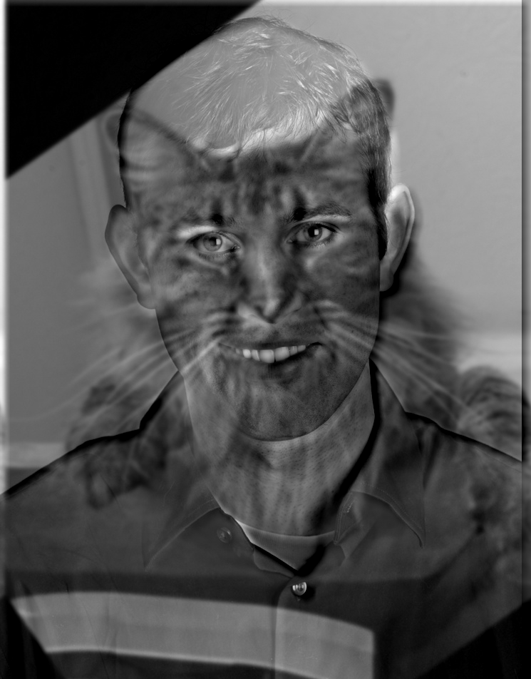
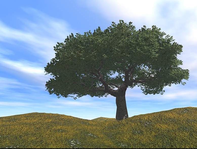
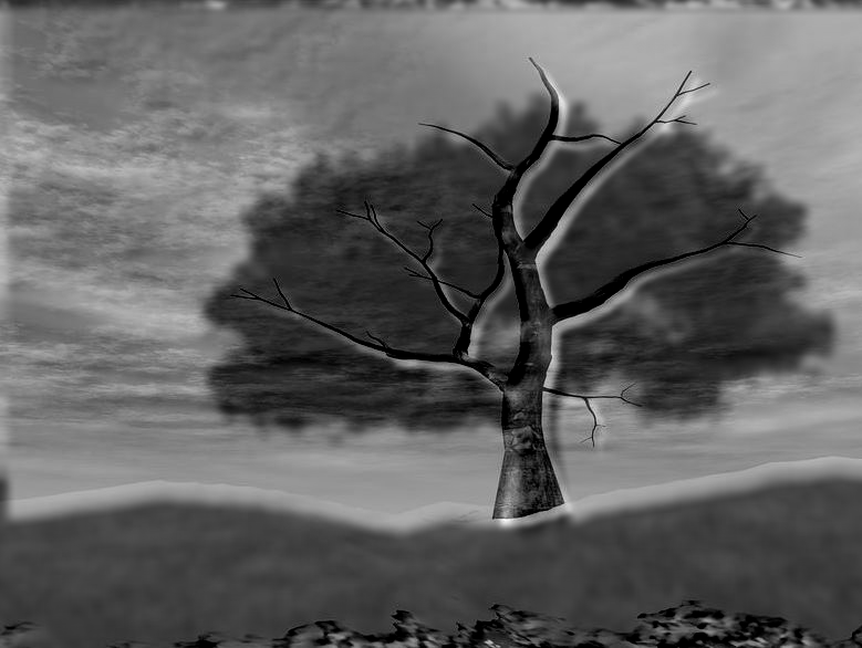
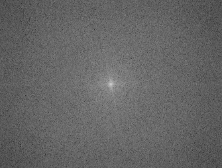
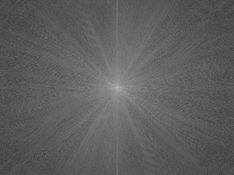
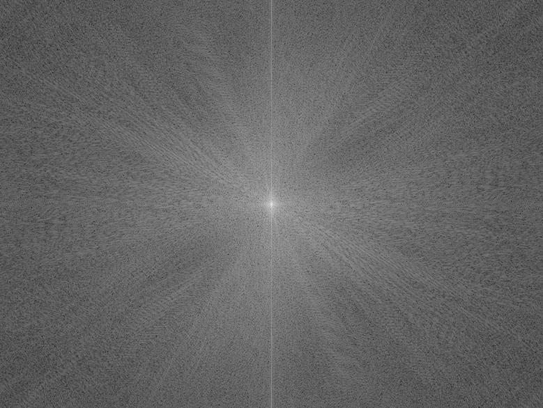
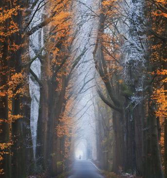
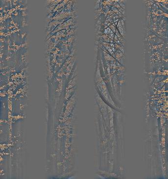
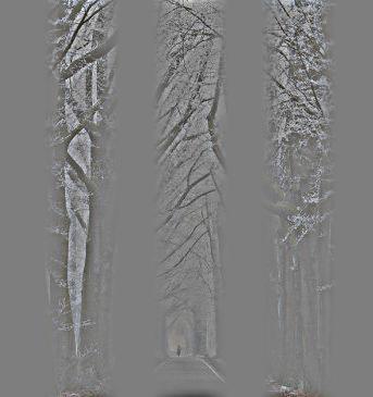
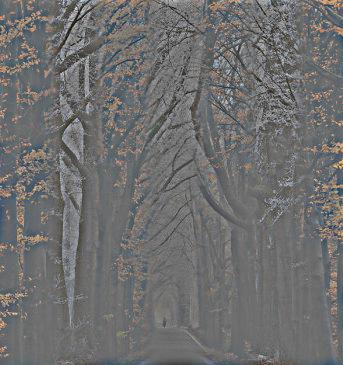
In the tree example below, the first input image already has relatively low frequencies and the second input image already has relatively high frequencies to begin with. When they are combined, the frequency plot looks similar to the second image, but is slightly brighter in the middle with the added lower frequencies from the first image. Because the second tree has such prominent high frequencies, it's still relatively visible at a distance.

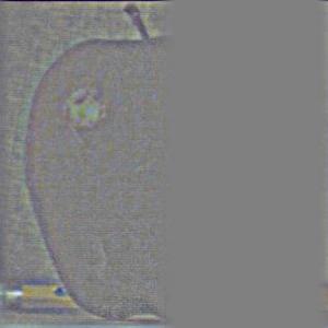
Part 2.3: Gaussian and Laplacian Stacks
For implementation of the Gaussian stack, I iteratively blurred through the image, such that the first image in the stack had one Gaussian applied, the second had two Gaussians applied (blurred twice), and so on until the Nth image had N Gaussians applied on it repeatedly.
For implementation of the Laplacian stack, I first computed a Gaussian stack of equal depth.
From there, each level of the Laplacian stack was computed using GaussianStack[i - 1] - GaussianStack[i],
where i represents the ith level of the Gaussian stack.
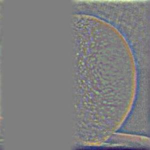
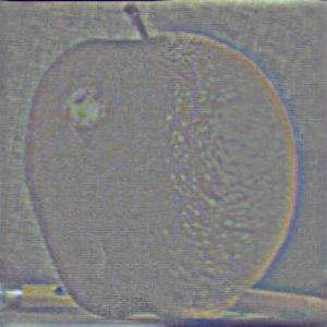
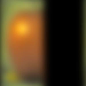
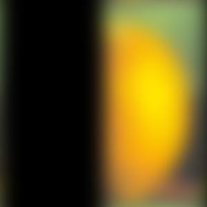
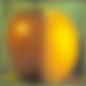
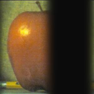
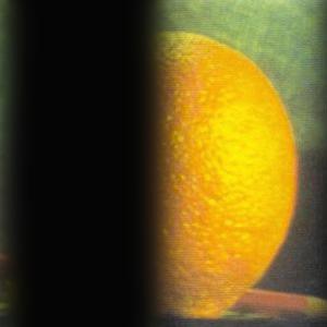
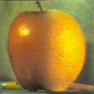
Below are the outcomes of the Laplacian and Gaussian stacks on the apple and orange to generate an oraple.
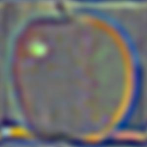
Part 2.4: Multiresolution Blending
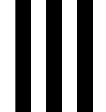
For implementation of multiresolution blending, I first constructed a mask that was used to blend the images, the basic one being a binary mask which is half white and half black. I then constructed a Gaussian stack of the mask, as well as 2 Laplacian stacks, one for each of the images being blended.
To combine the image, for each stack level I combined the two images with the computation of mask * Laplacian(i) for image 1 + (1 - mask) * Laplacian(i) for image 2, where Laplacian(i) represents the ith layer of the Laplacian stack for the image. I then summed up these values across all levels to yield the final blended image.

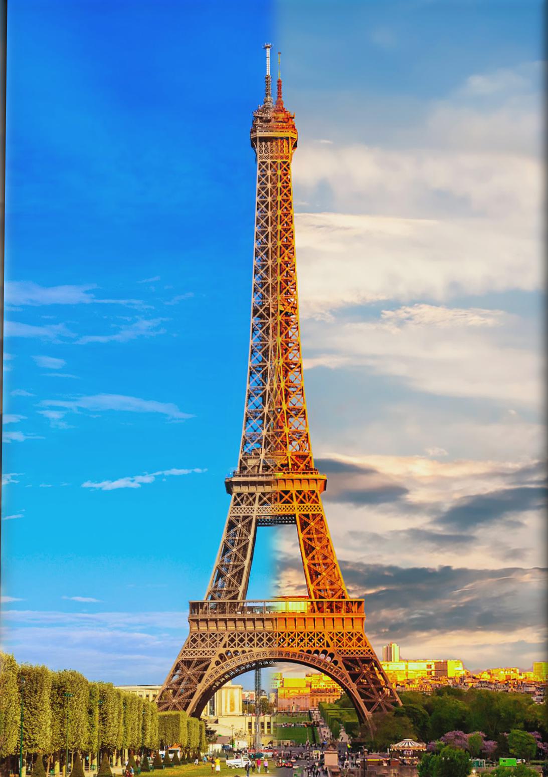
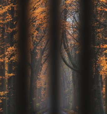
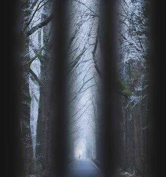
Irregular mask 1: Stripes
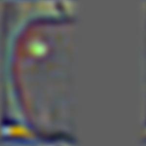
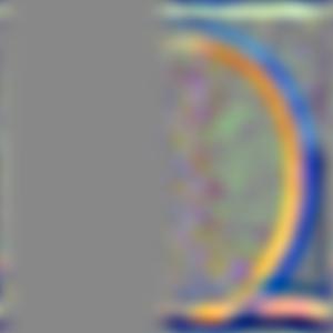
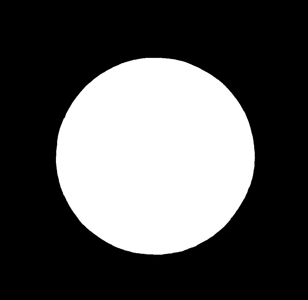
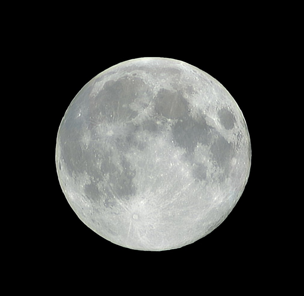
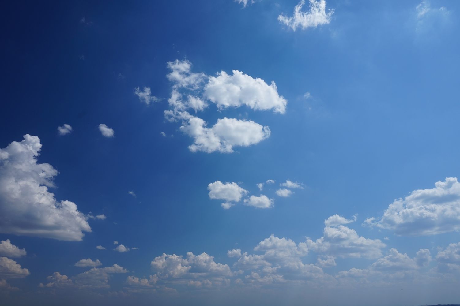
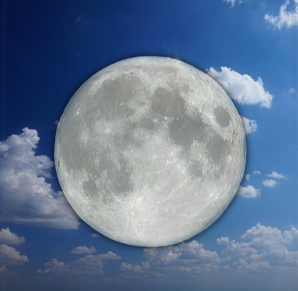
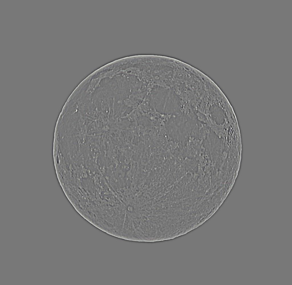
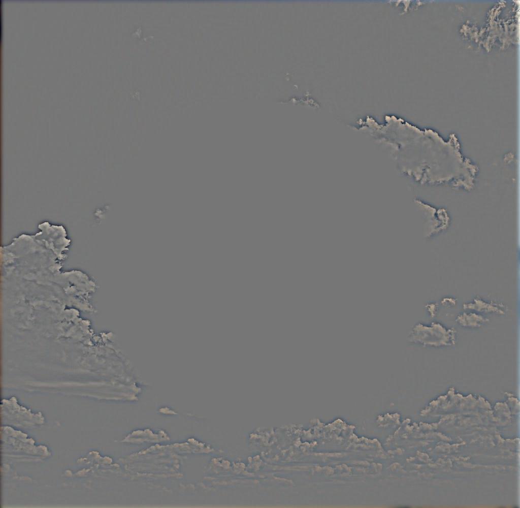
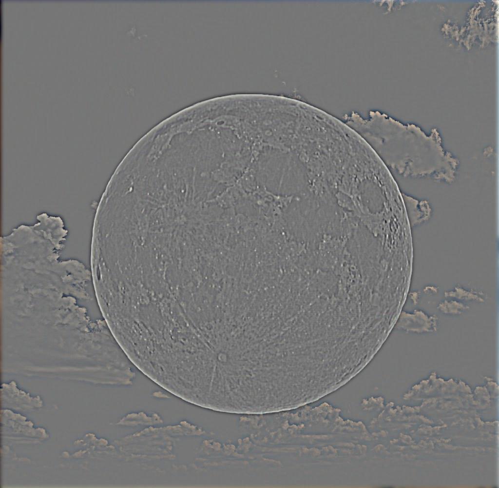
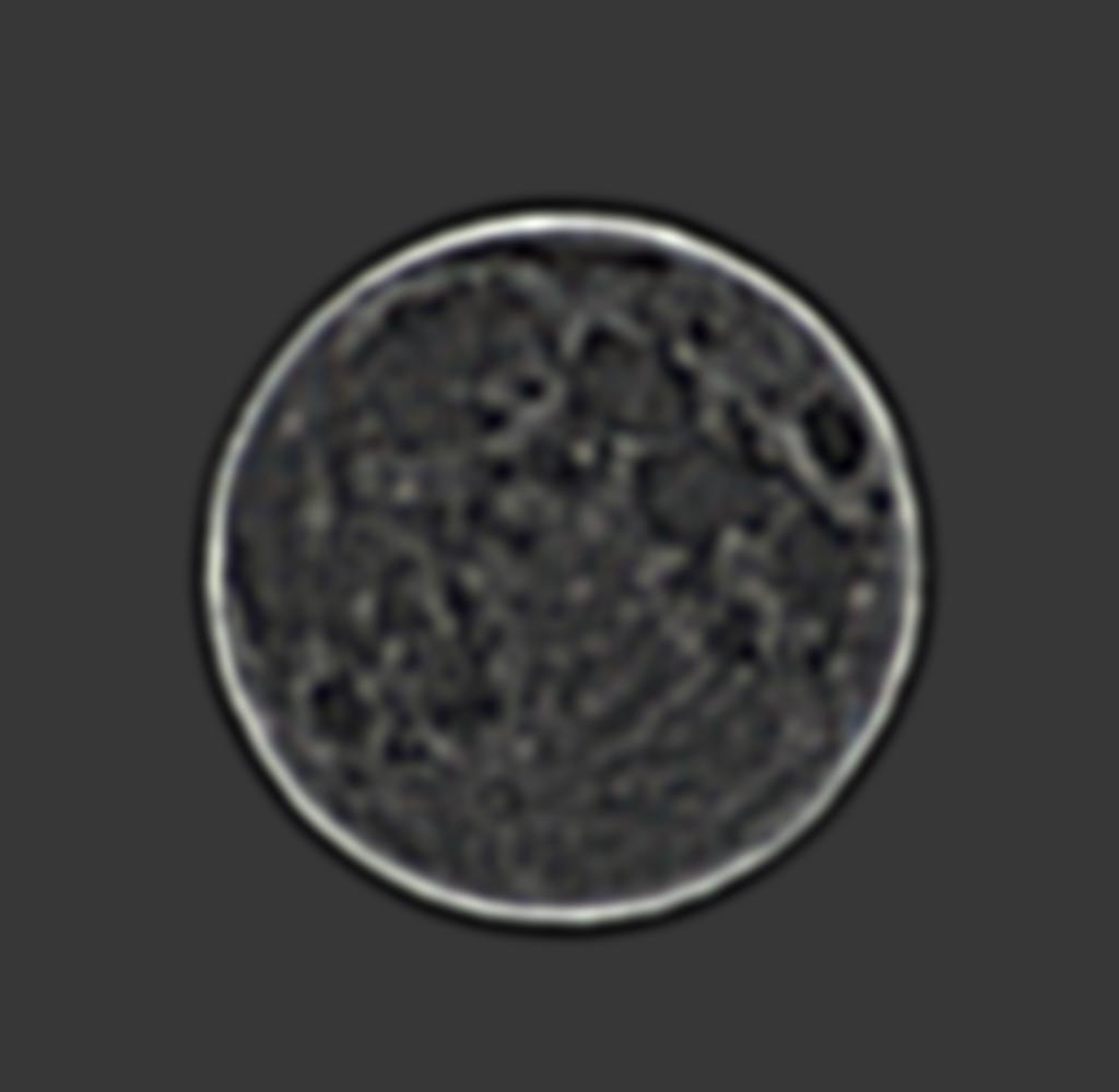
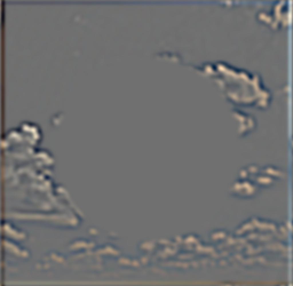
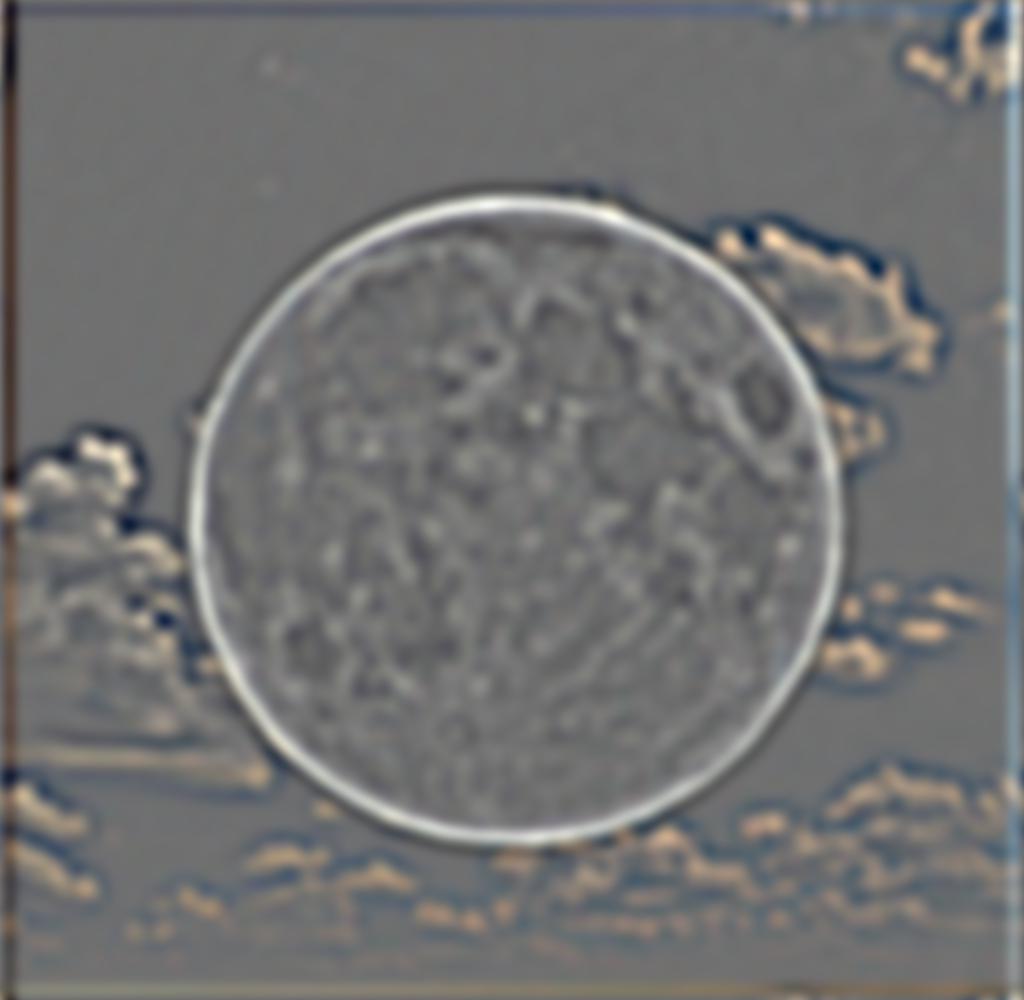
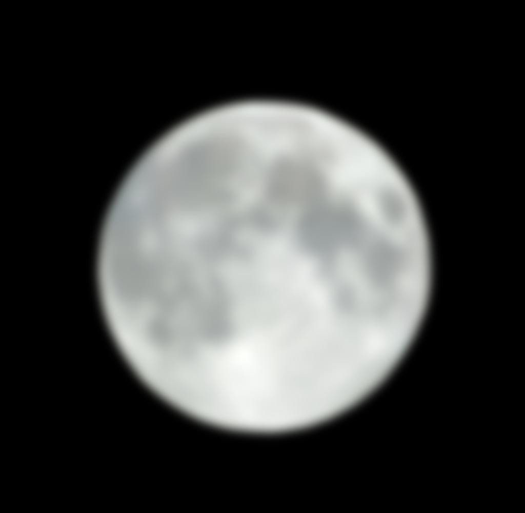
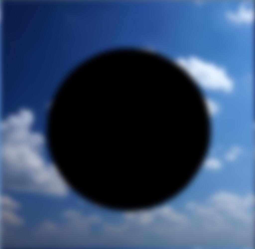
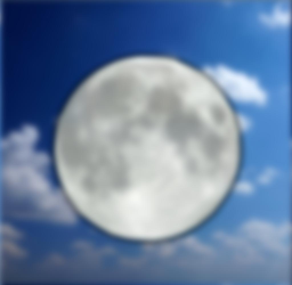
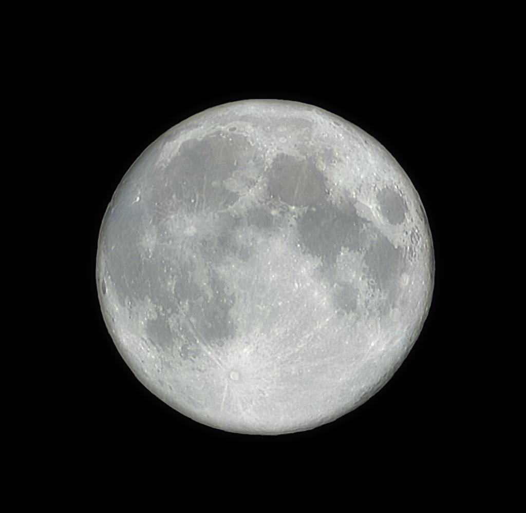
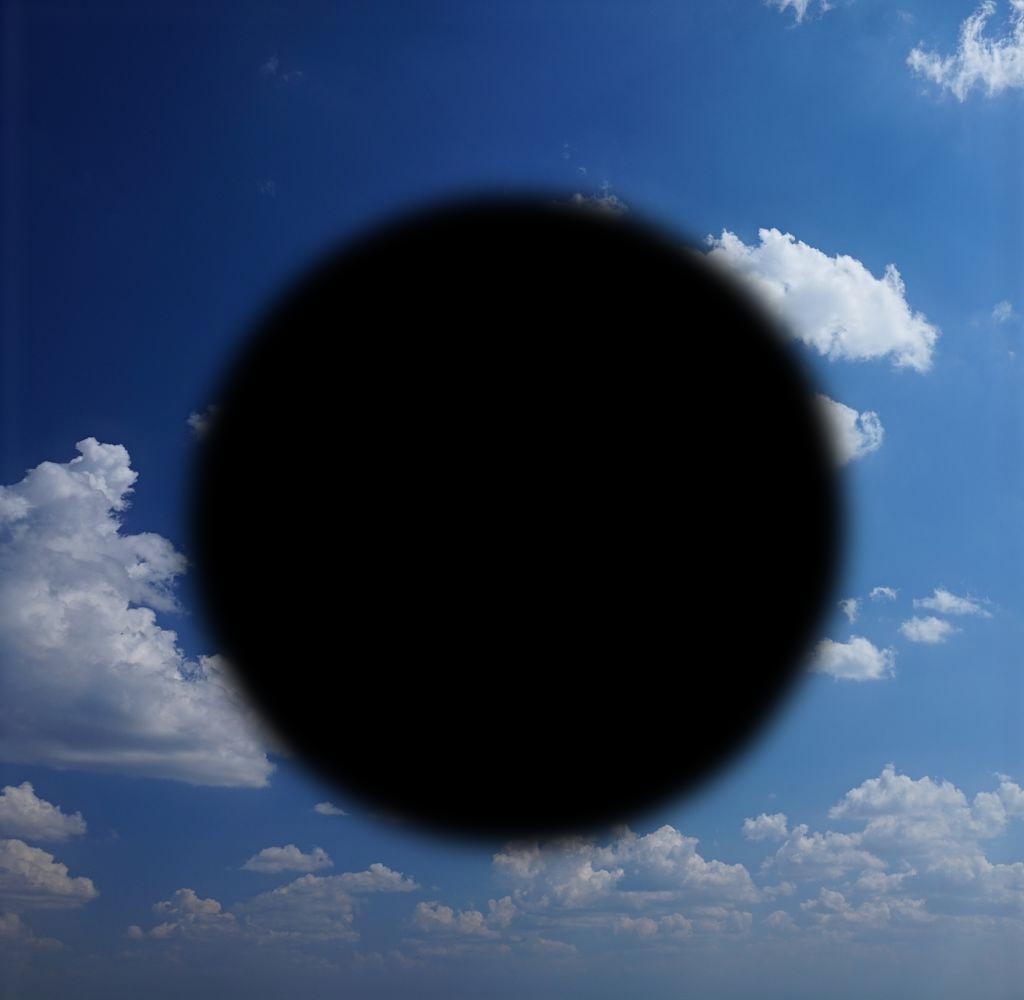
Irregular mask 2: Circle
For another irregular mask I used a circle, which I generated using the moon image below and binarizing it. From there I applied the blending, which results in a drop shadow look behind the moon, blending the black background from the moon onto the sky background.
Takeaways
One important thing I learned from the project was how Gaussian and Laplacian stacks work in tandem, especially with splines. The Gaussian stack is useful for applying a gradual blur across a mask rather than clear defined lines because of how it removes the high frequencies, while the Laplacian stack is useful in extracting ranges of frequencies.