Project 2: Fun with Filters and Frequencies!
COMPSCI 194-26: Computational Photography & Computer Vision (Fall 2021)
Alina Dan
Fun with Filters
Part 1.1: Finite Difference Operator
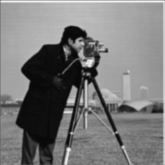
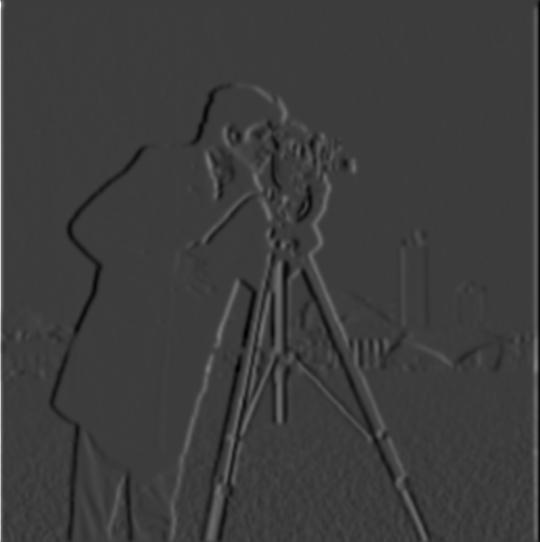
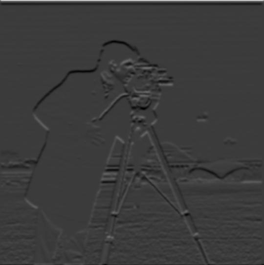
To show the partial derivatives in x and y of the cameraman image, I convolved the image with finite difference filters:
Dx = [1, -1]
Dy = [[1], [-1]]
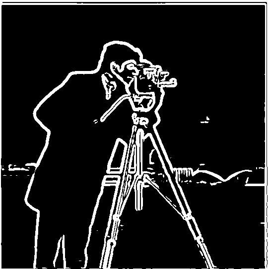
I then computed the gradient magnitude through taking the root of dx⁄dt2 + dy⁄dt2 (i.e the root of the sum of squares of the partials).
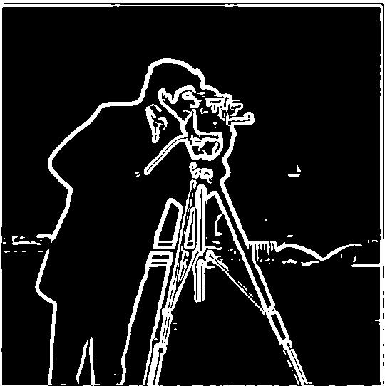
Following that, I binarized the gradient magnitude to get an edge image. This is done through picking some threshold of which noise should be removed.
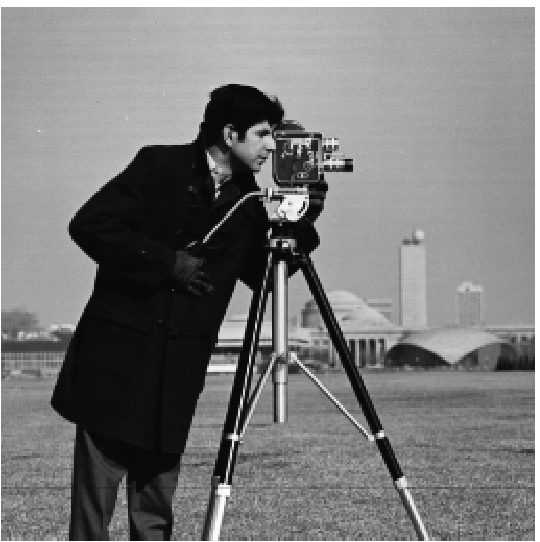 Cameraman Photo
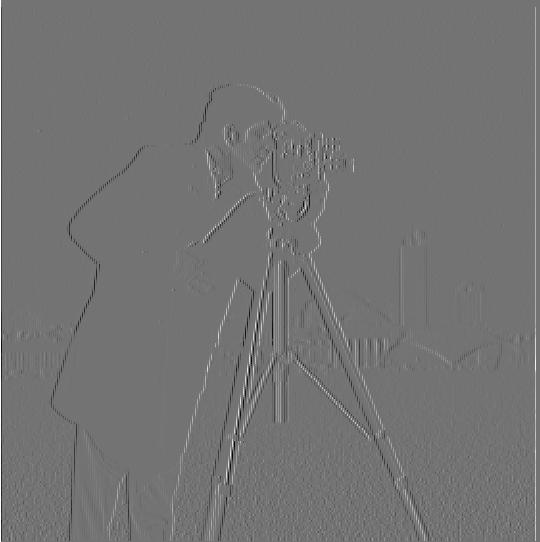 Partial X
|
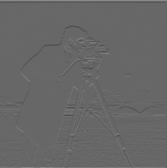 Partial Y
|
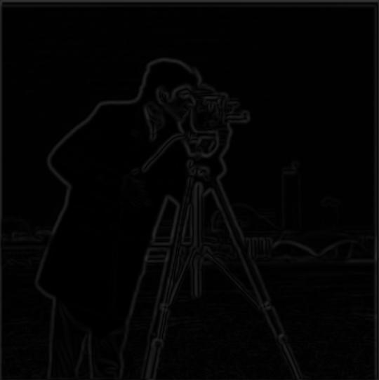
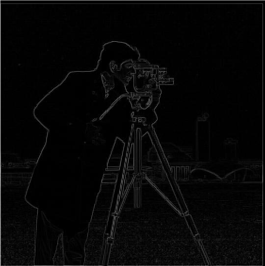 Gradient Magnitude
|
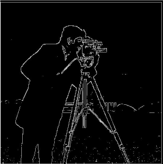 Binarized Gradient Magnitude
|
Part 1.2: Derivative of Gaussian (DoG) Filter
For this section, prior to computing the partials, gradient magnitude, and edge image, I blur the cameraman photo first. I do this by convolving the original image with a Gaussian. The steps afterwards follow the same logic as that from the above section (1.1).
 Blurred Cameraman Photo
 Blurred Partial X
|
 Blurred Partial Y
|
 Blurred Gradient Magnitude
|
 Blurred Binarized Gradient Magnitude
|
Comparing the result from convolving with a Gaussian versus not, the edges of the blurred edge image are more solid and pronounced. Accompanying this, the edges are thicker due to the blur. We also see less noise in the blurred edge image than the non-blurred edge image (most noticeable towards the bottom edge of the photo) despite utilizing the same noise threshold.
One Convolution
Iterating off of the above, we can actually accomplish the same thing through only _one_ convolution! Rather than convolving the original image with a Gaussian first, we can convolve the Gaussian with the finite difference operators first. Afterwards, we can convolve that resulting filter with the cameraman image. We can actually see that whether we convolve the image with the Gaussian first or we convolve the Gaussian with the finite difference operators first, we get the same result.
 Gaussian Convolved with Dx
|
 Gaussian Convolved with Dy
|
 Gradient Magnitude
|
 Binarized Gradient Magnitude
|
Fun with Frequencies
Part 2.1: Image "Sharpening"
Given a blurry image, we can actually "sharpen" it through utilizing the unsharp marking technique. First, we use a low pass filter (Gaussian) on the blurred image to get the low frequencies. We then subtract the low frequencies from the blurred image, leaving the high frequencies. We then add some (alpha * high frequencies) to the blurred image because images look sharper with more high frequencies.
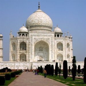 Blurry Taj
|
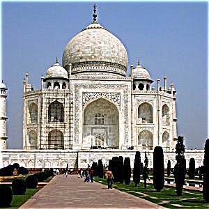 Sharpened Taj
|
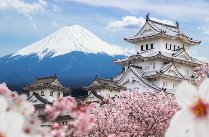
To see the full effects and capabilities of the unsharp mask, I took some clear photos, blurred them with a Gaussian filter, and then applied the unsharp mask.
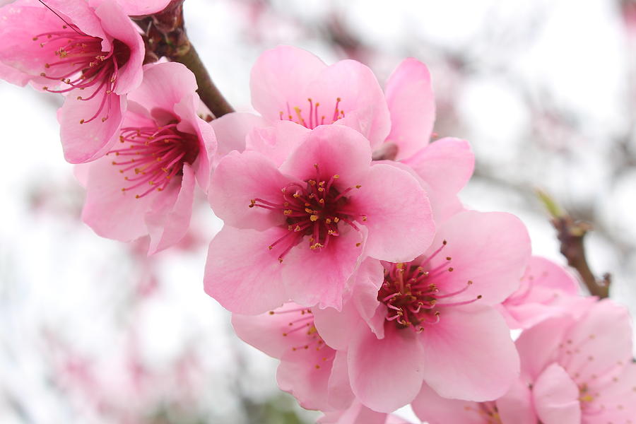 Original Cherry Blossoms
|
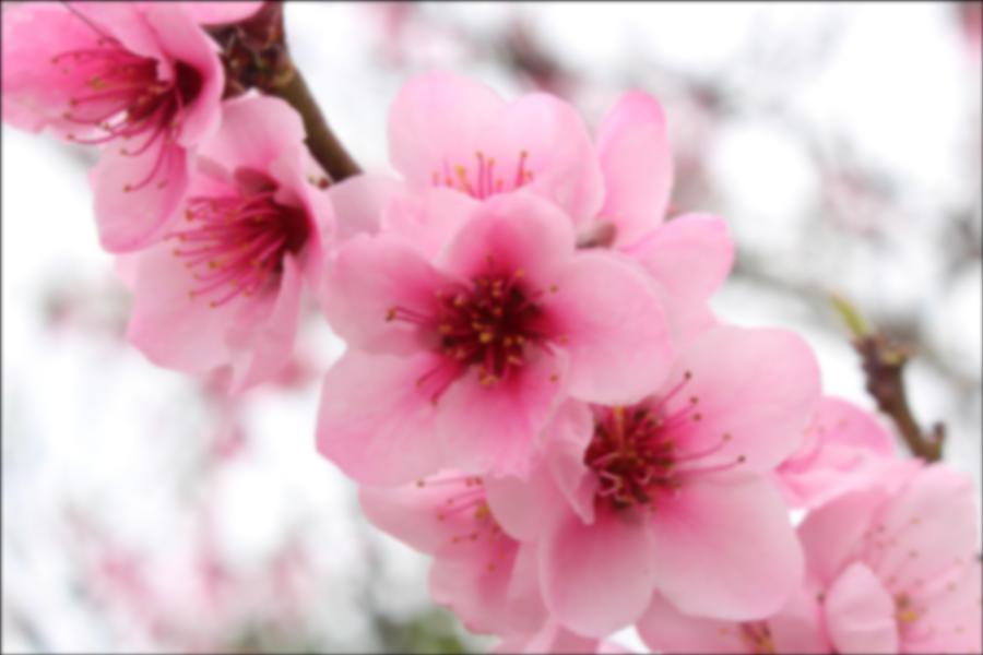 Blurred Cherry Blossoms
|
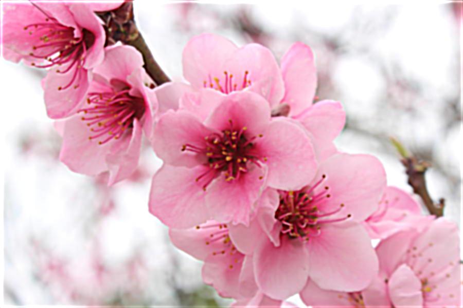 Sharpened Cherry Blossoms
|
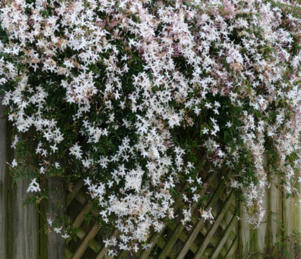 Original Jasmine
|
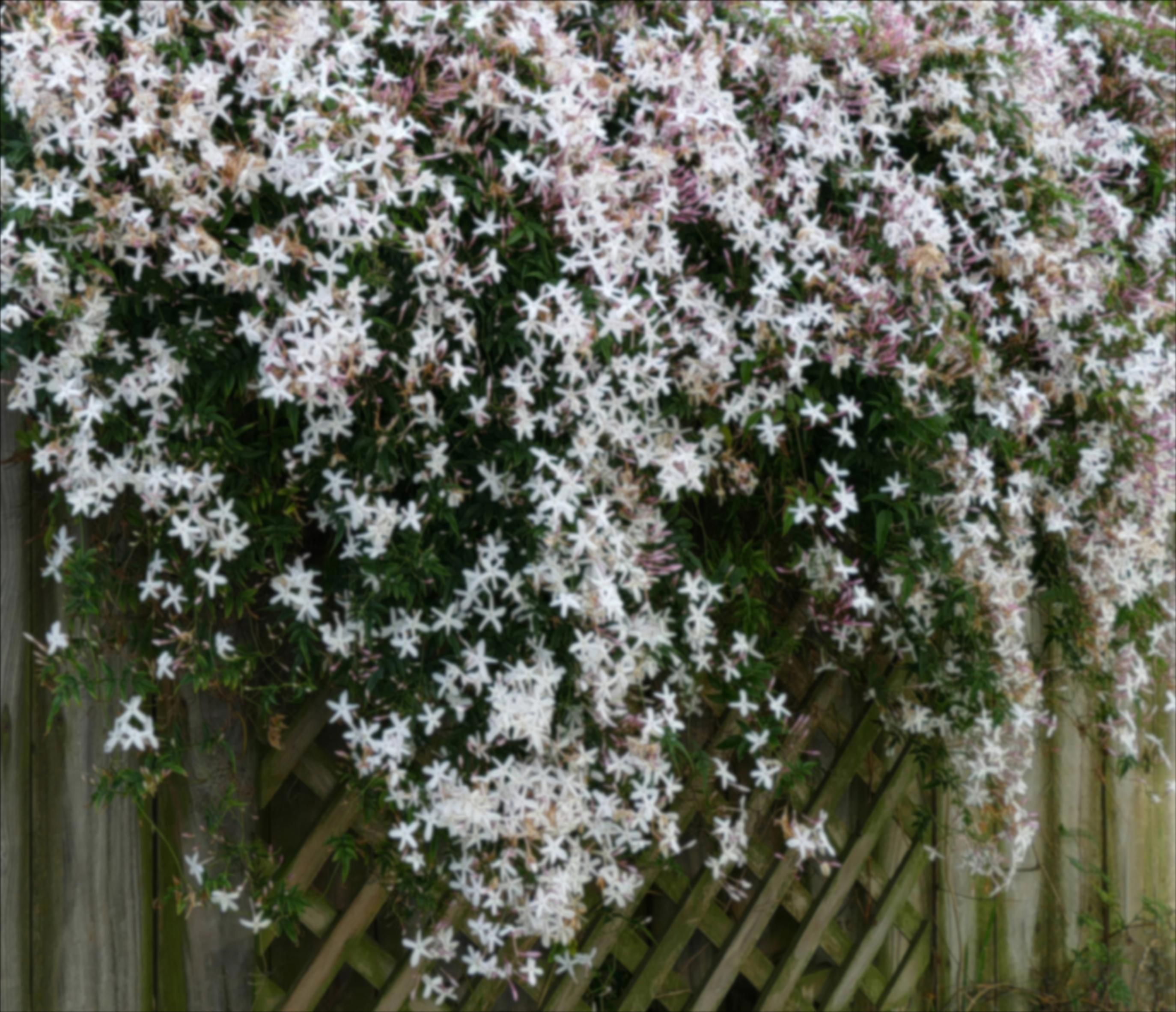 Blurred Jasmine
|
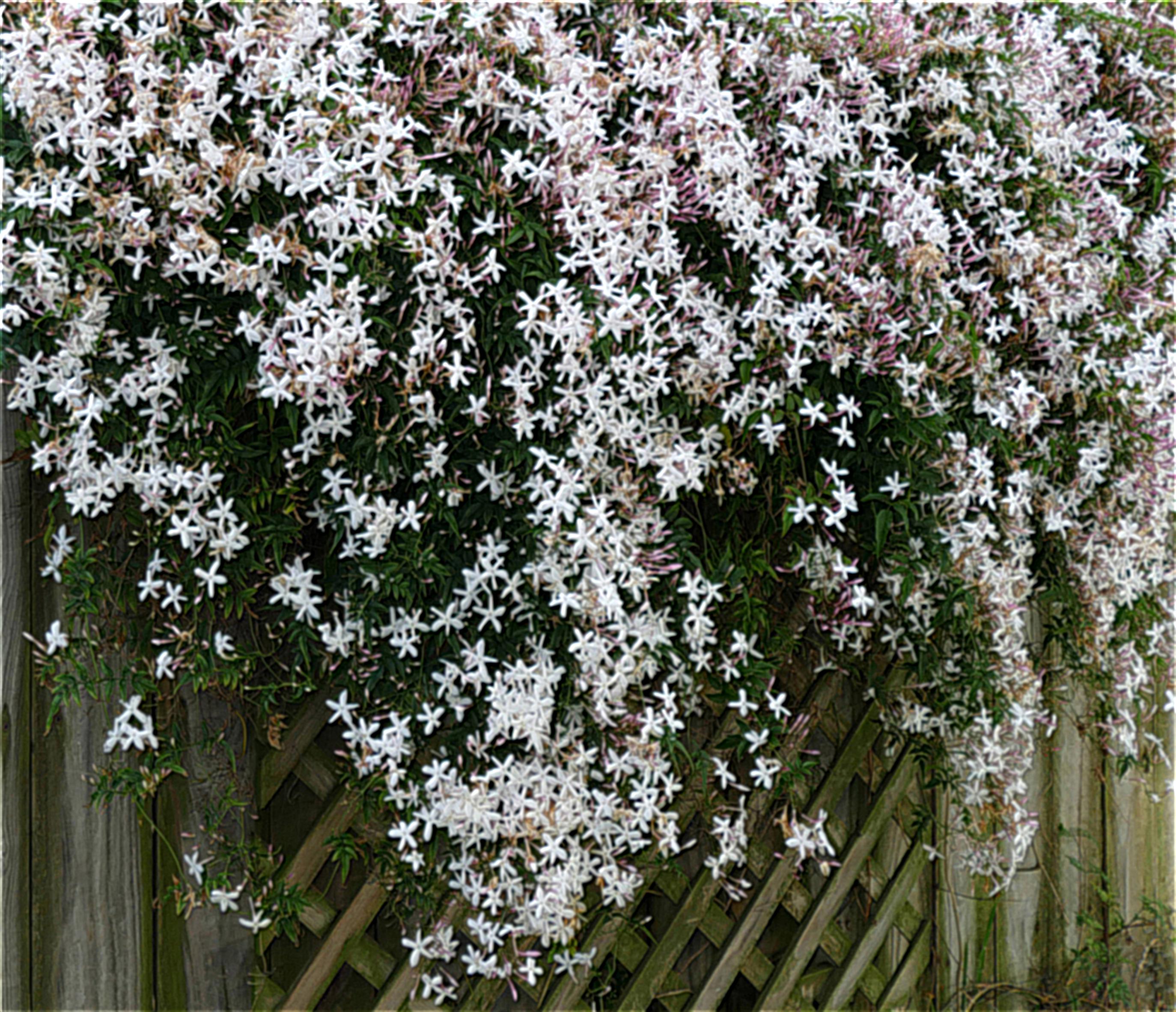 Sharpened Jasmine
|
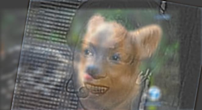
Part 2.2: Hybrid Images
By blending the low frequencies of one image with the high frequencies of another image, we can create hybrid images. Specifically, the low frequencies are taken from a low pass filter (Gaussian) on an image, and the high frequencies are taken from subtracting the low frequencies from the original image.
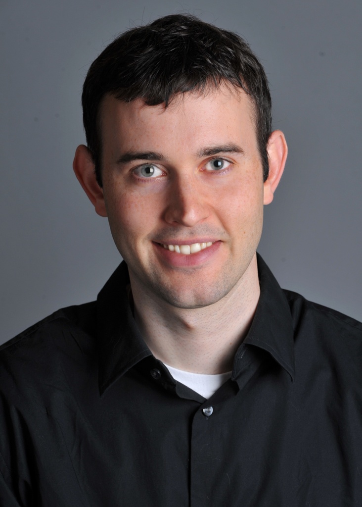 Derek
Derek
|
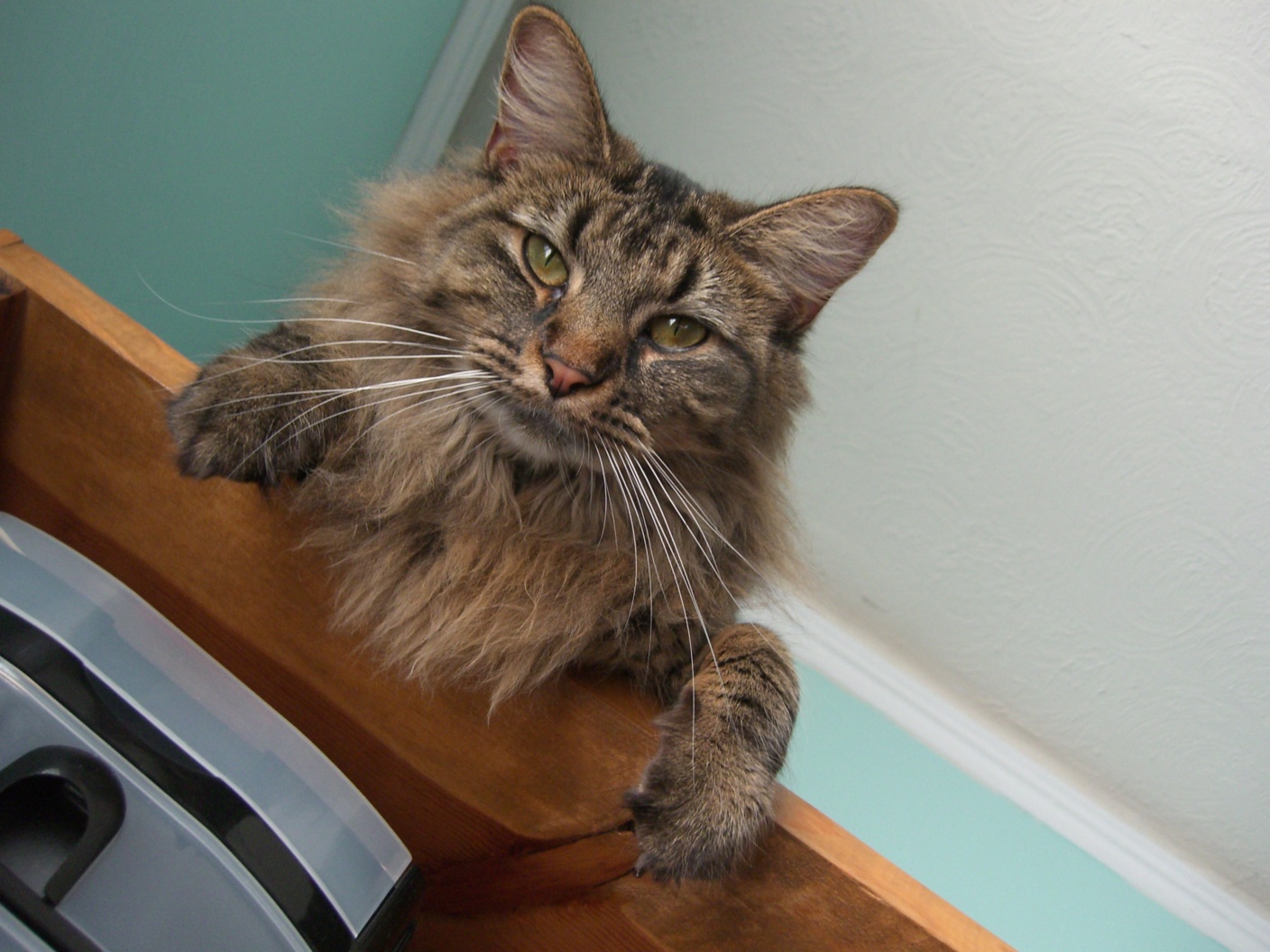 Nutmeg
|
 Derek Nutmeg Hybrid
|
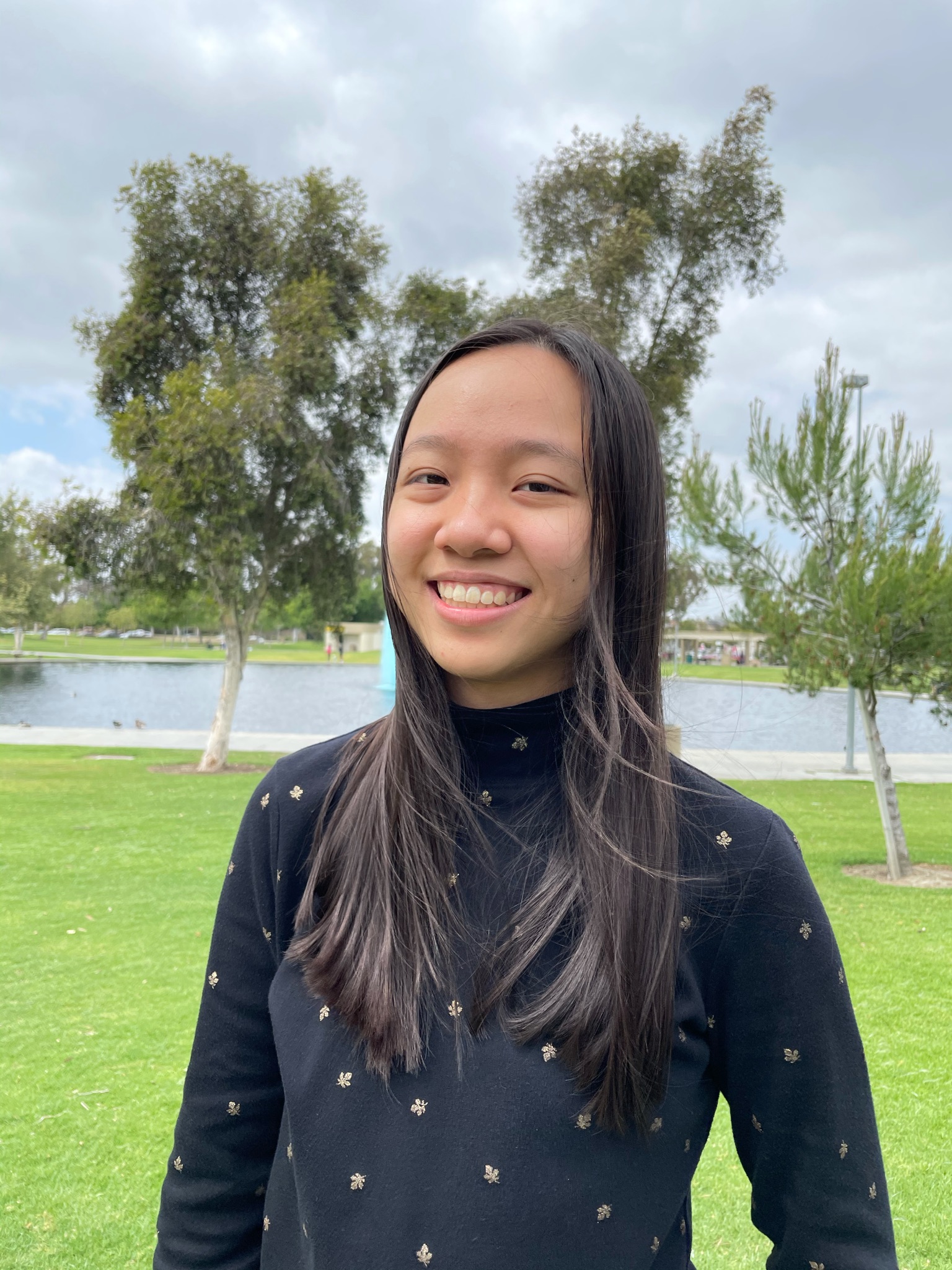 Malleeka
|
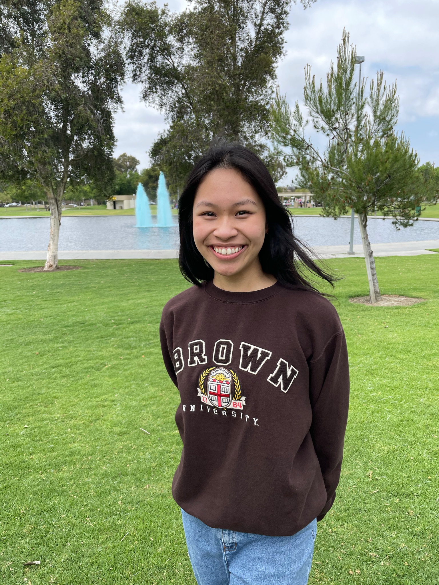 Rachel
|
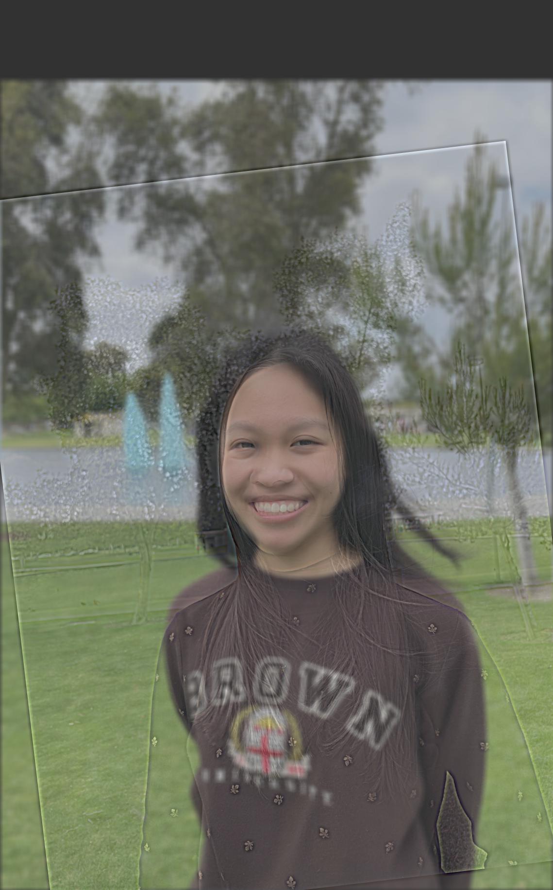 Malleeka Rachel Hybrid
|
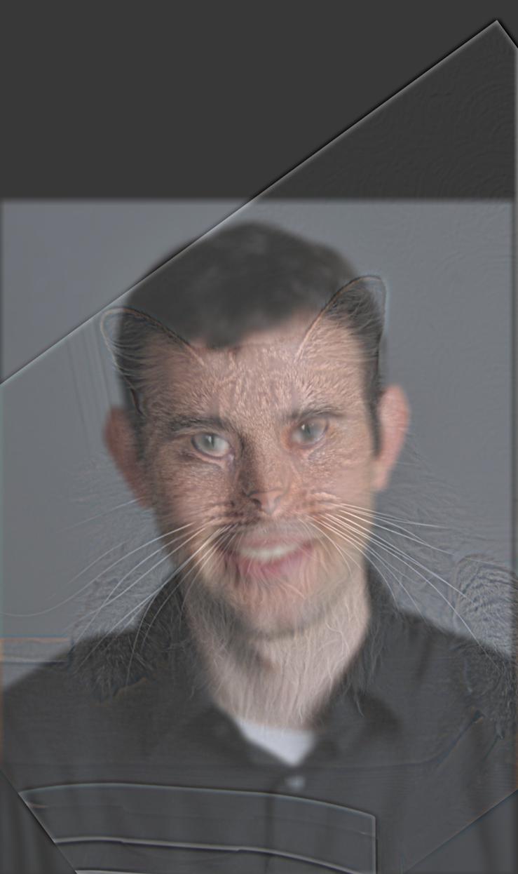
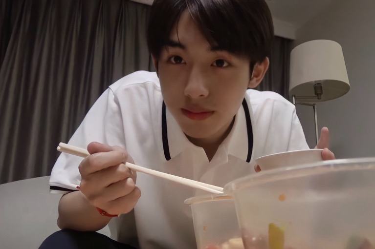 Winwin
|
 Smiling Winwin
|
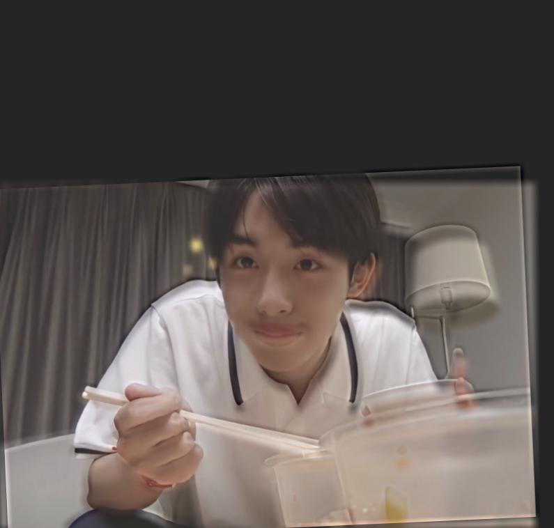 Winwin Expression Hybrid
|
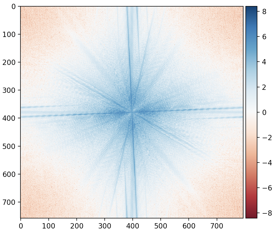
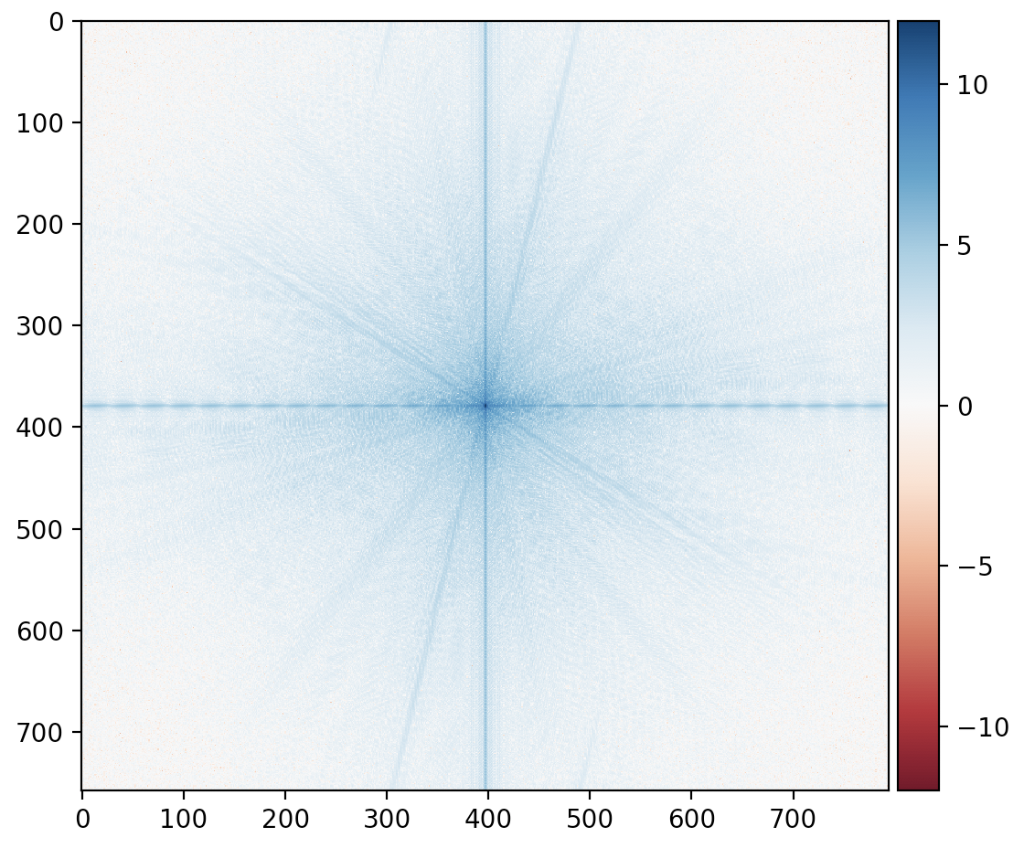 Winwin Fourier
|
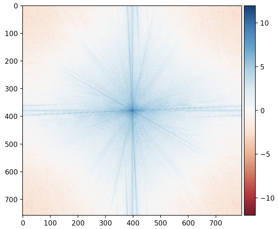
 Smiling Winwin Fourier
|
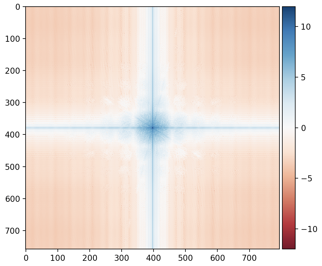 Low Pass Winwin Fourier
|
 High Pass Smiling Winwin Fourier
|
 Winwin Expression Hybrid Fourier
|
Failure
I attempted to merge a deer with a singer, but the pictures did not align well due to the extremely differing shapes of facial features. It is difficult to see the pudu and it doesn't seem to blend the two pictures together well.
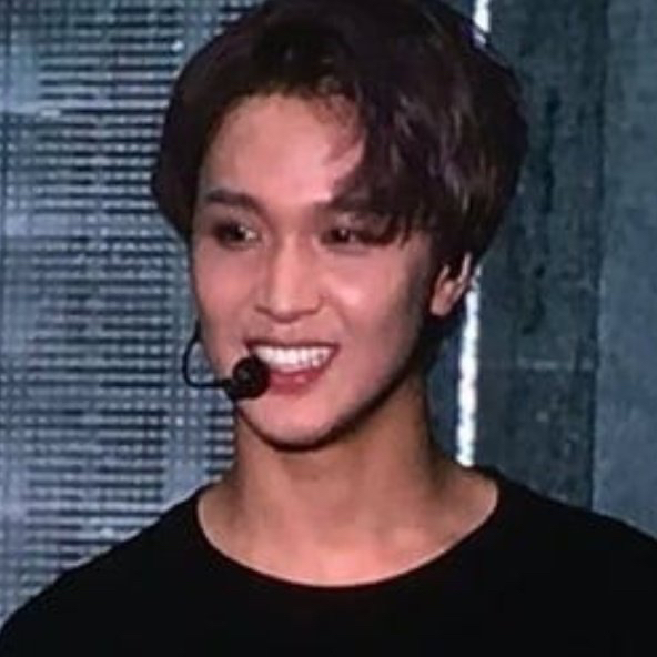 Haechan
|
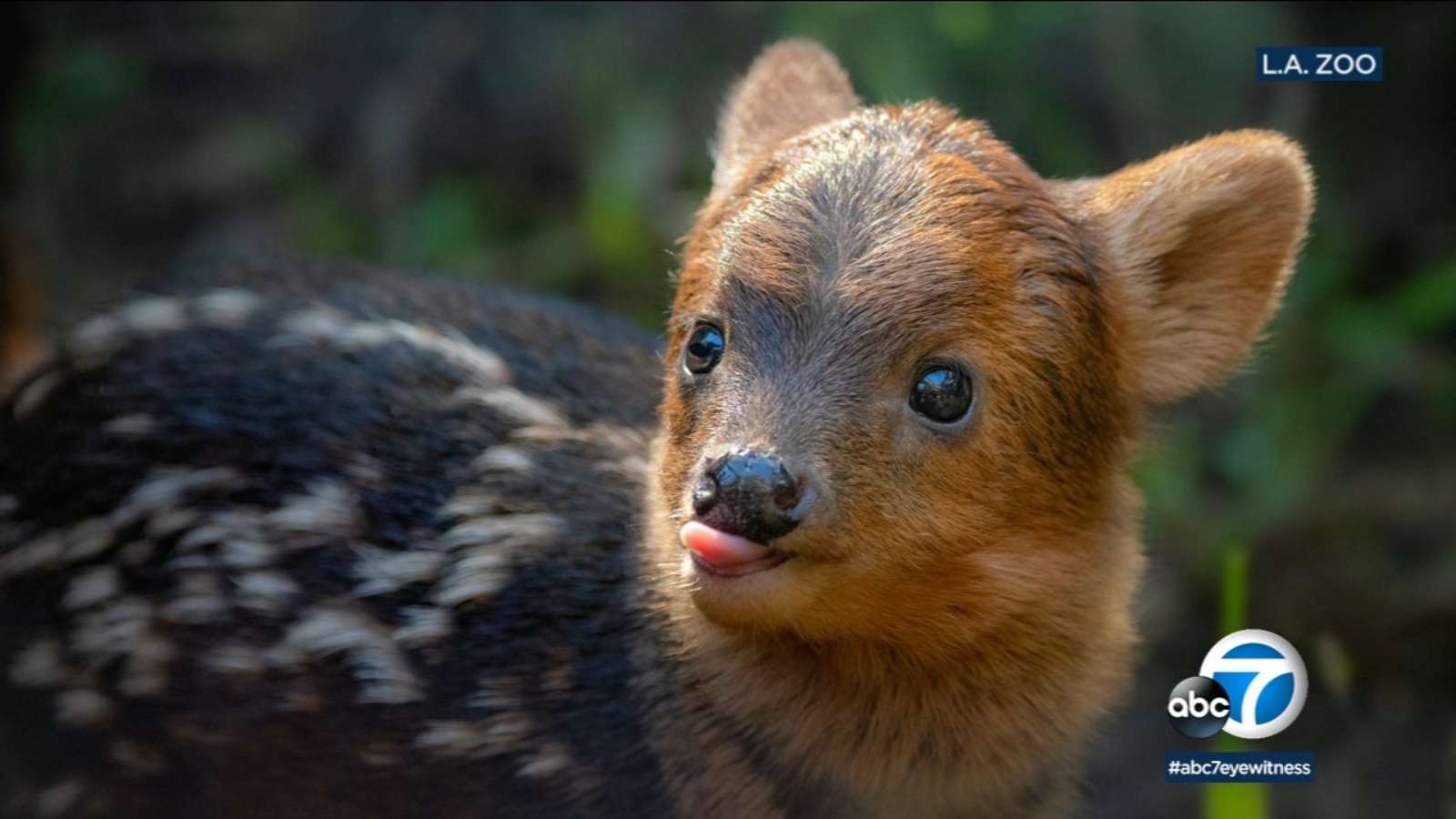 Pudu
Pudu
|
 Haechan Pudu Hybrid
|
Bells & Whistles
I implemented color images for both low and high frequency images to see if hybridization would work better compared to greyscale images. It seems that the hybridization works well with color images due to enhancing the clarity of both low and high frequency images.
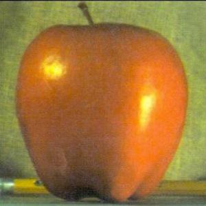
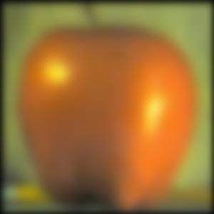
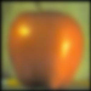
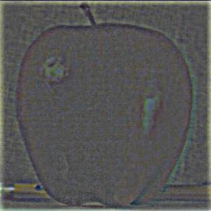
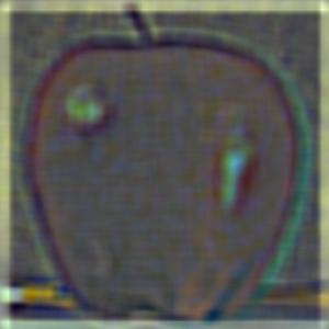
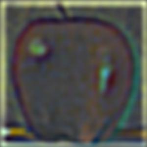
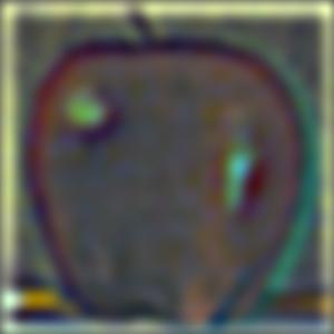
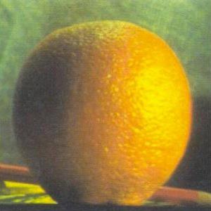
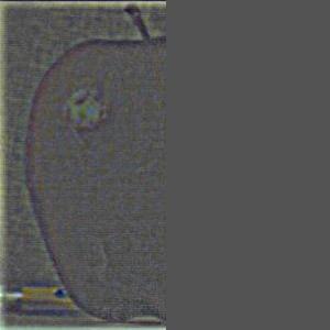
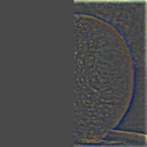
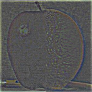
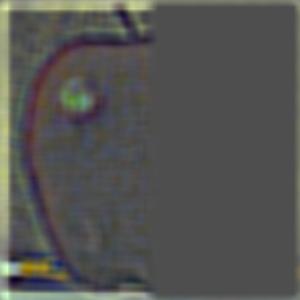
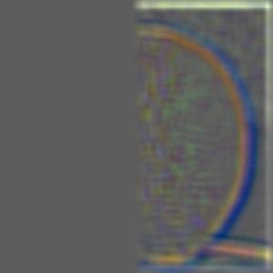
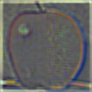
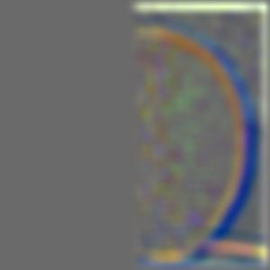
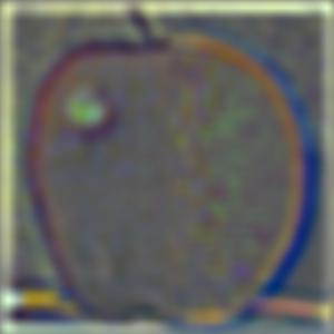
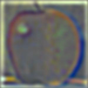
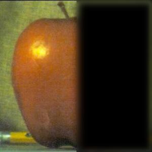
Part 2.3: Gaussian and Laplacian Stacks
Implementing a Gaussian stack involves taking an image, convolving it with a Gaussian, convolving that resulting image with a Gaussian, so on and so forth. Thus, on each layer, a Gaussian filter is applied to the previous layer's output. With a Laplacian stack, we take the difference between pairs of the Gaussian stack layers. The last Laplacian stack layer is the same as that of the Gaussian stack last layer. In particular, I used N = 5 for the number of levels in my stacks.
Gaussian Stack for the Apple
Laplacian Stack for the Apple
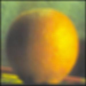
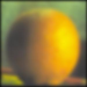
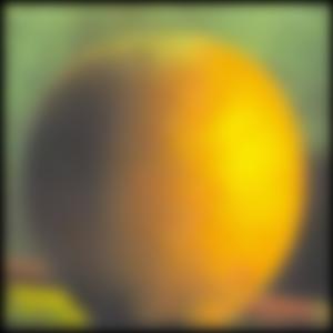
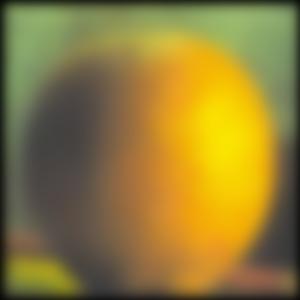
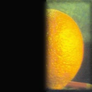
Gaussian Stack for the Orange
Laplacian Stack for the Orange
c
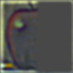
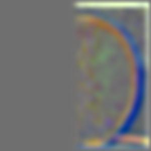
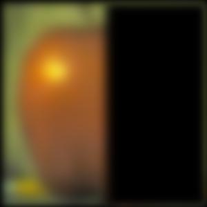
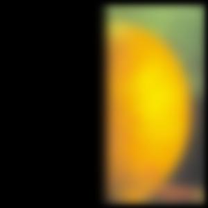
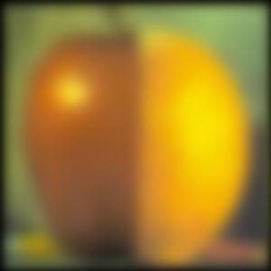
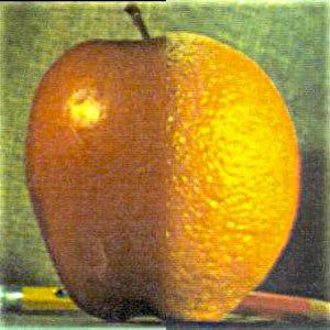
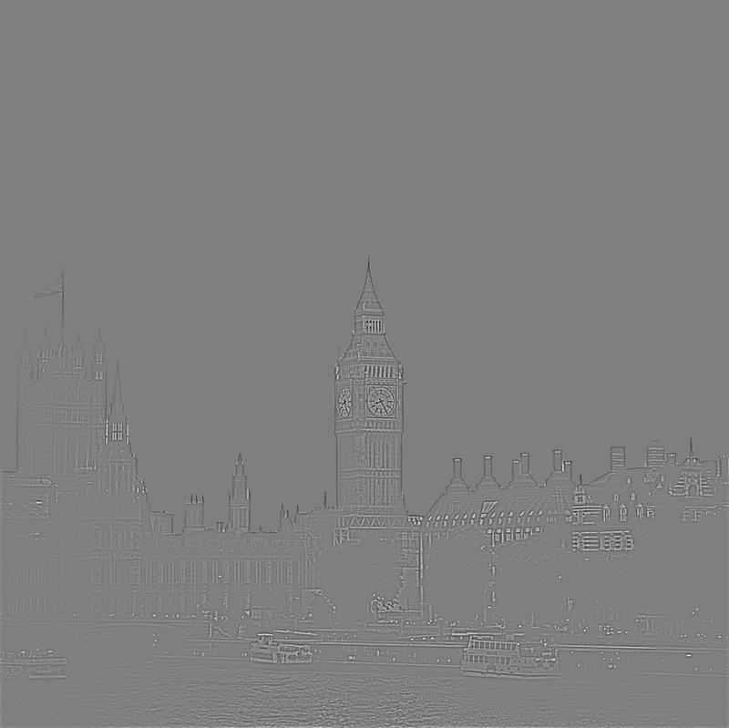
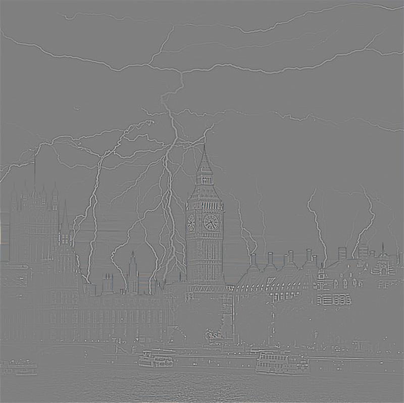
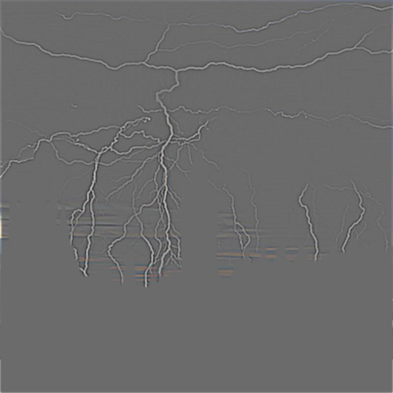
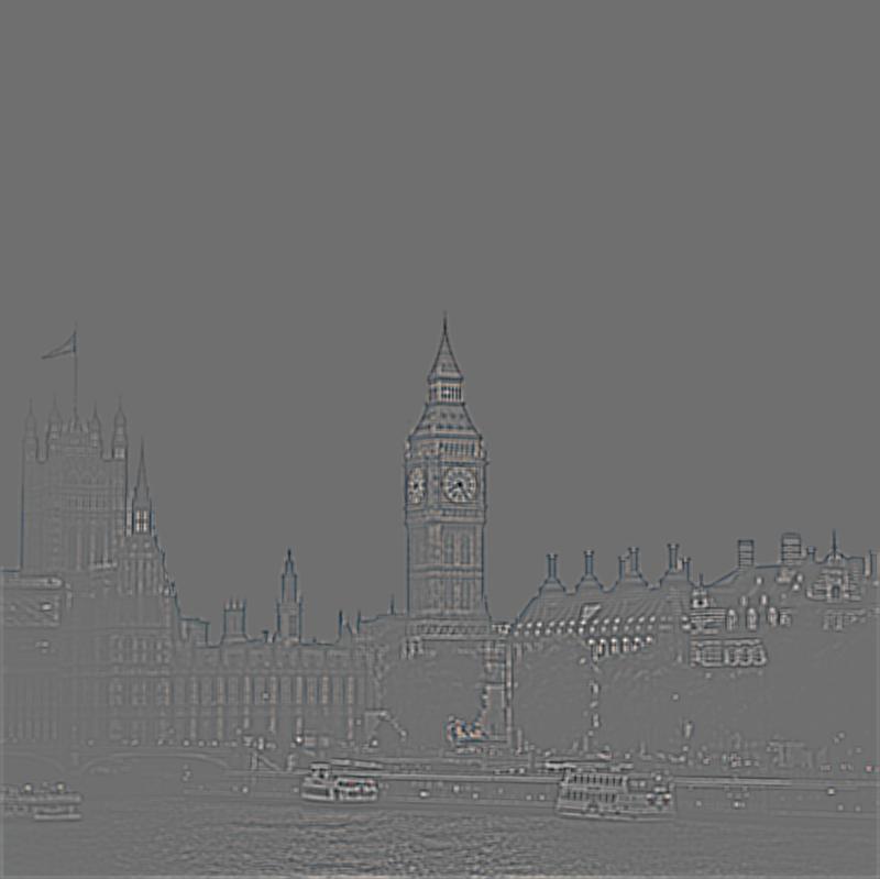
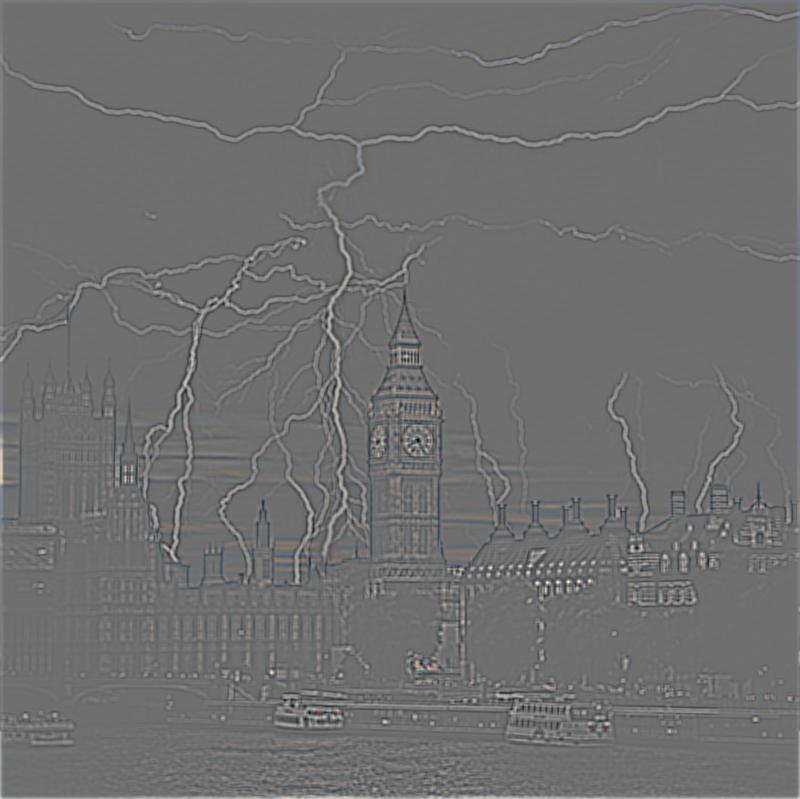
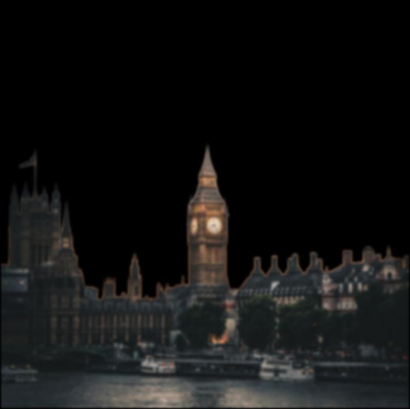
Part 2.4: Multiresolution Blending (a.k.a. the oraple!)
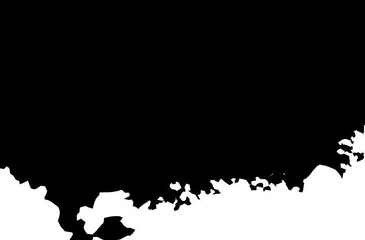
Following from the previous section of building Laplacian stacks for the orange and apple image, I then generated a Laplacian stack based on the combination of the two stacks. For the blending, I created a mask and generated a Gaussian stack for the mask. To get the finalized blended image, I summed over all levels of the combined Laplacian stack.
| Gaussian Mask on Apple |
Gaussian Mask on Orange |
Sum of Column 1 and 2 |
|
|
|
|
|
|

|
|
|
|
|
|
|
|
|
|
|
|
|
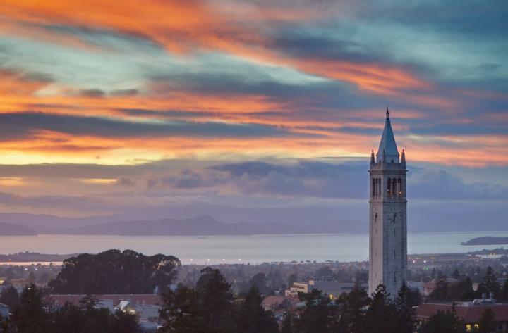
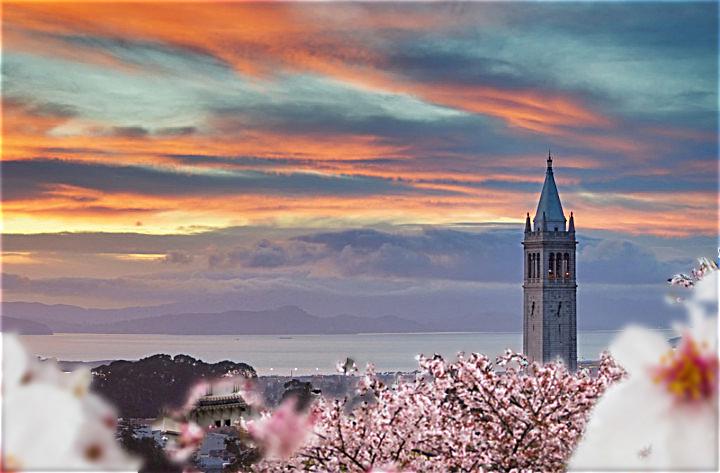
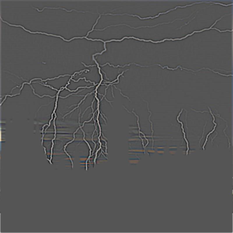
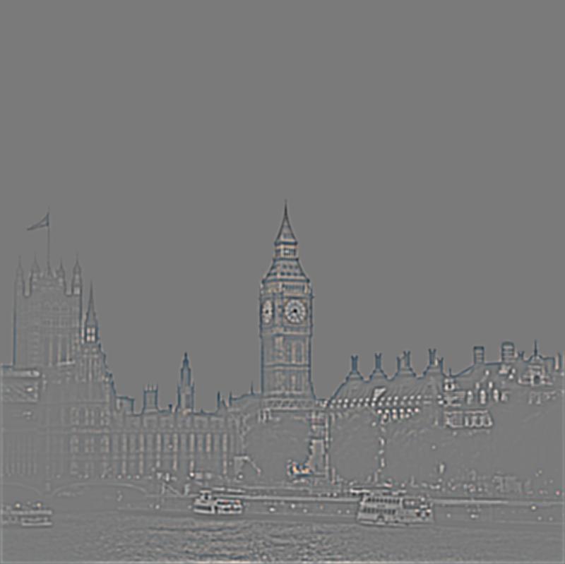
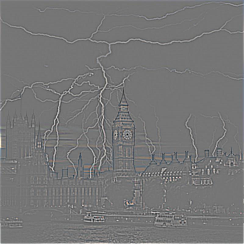
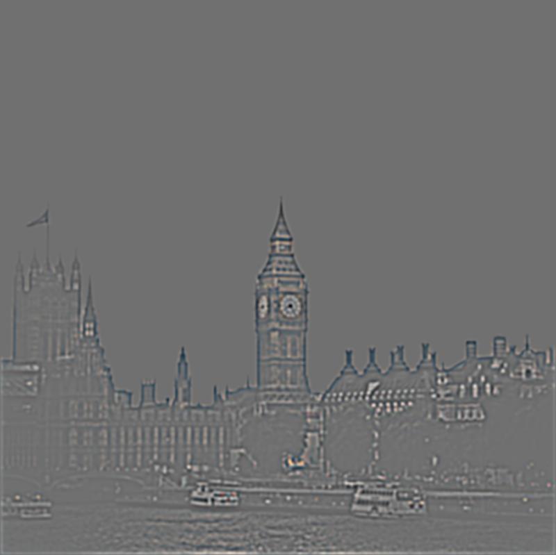
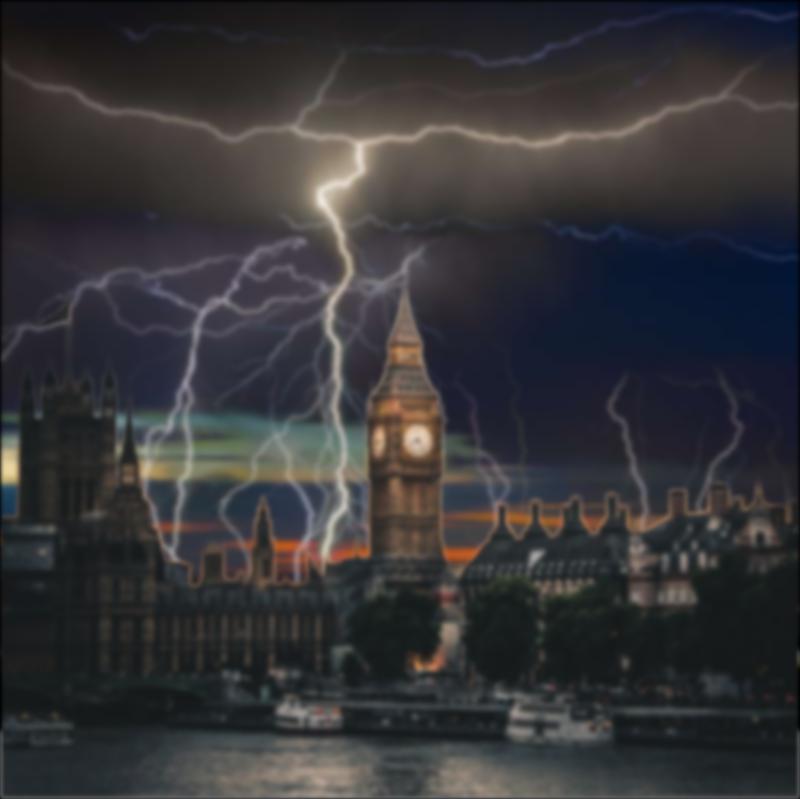
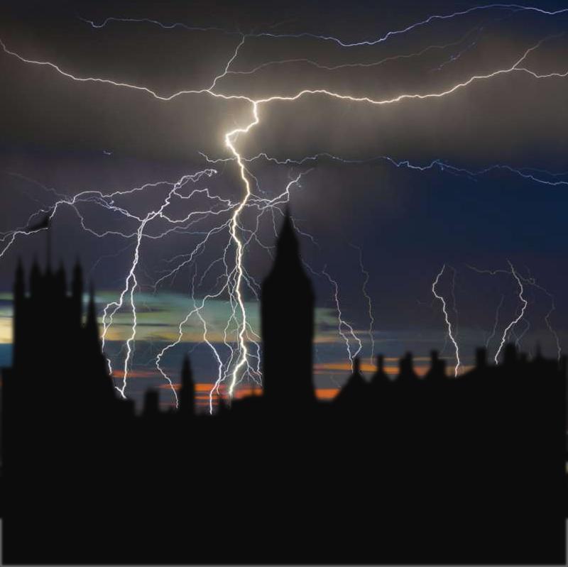
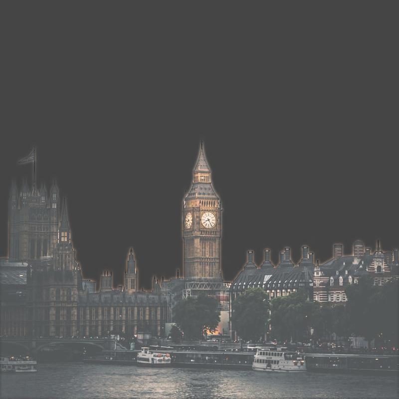
| Gaussian Mask on London |
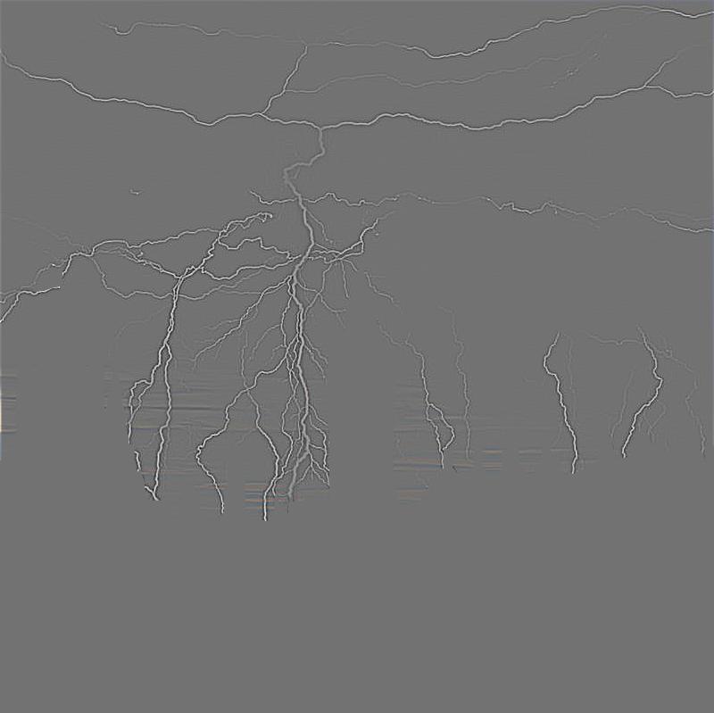
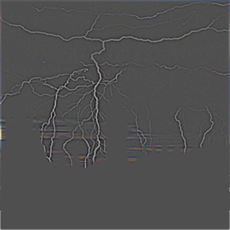
Gaussian Mask on Lightning |
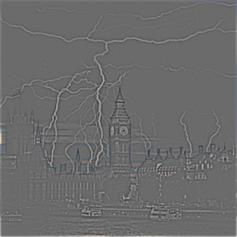
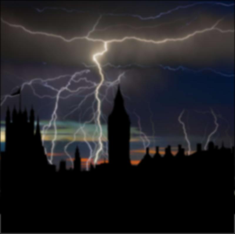
Sum of Column 1 and 2 |
|
|
|
|
|
|
|
|
|
|
|
|
|
|
|
|
|

|
Bells & Whistles
Rather than working with only greyscale images, I incorporated color images for the blending. With this, it is much easier to visually see the blending of images due to greater distinguishability within images. To implement this, I separated images into their respective R, G, and B channels, used the blending logic on each channel invidually, and then stacked the channels together to get the finalized color image.
Learnings
In terms of what I learned, I found the most interesting thing to be finding out that there are many factors that play into whether an operation turns out "good" or not. For example, in the hybrid images, I found out through trial and error that some images shouldn't be merged together due to orientation of the images (ex. someone's face is turned a certain direction), color scheme of the image, and more. Another example is that in the blending section of this project, despite there being a lot of cool ideas of blending different images, sometimes they just don't turn out nice. This may be due to factors such as limitations in the blending, frequency differences, and color. There actually should be a lot of thought put into picking pictures to operate and perform on.