Project 2. Fun with Filters and Frequencies!

Part 1.1. Finite Difference Operator

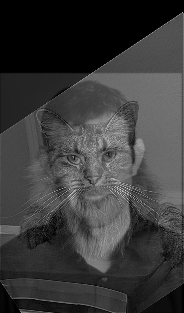
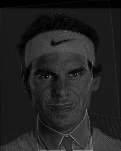
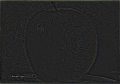
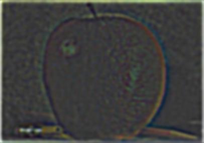
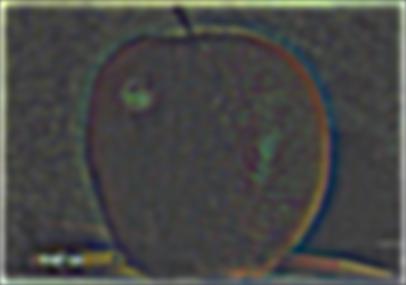
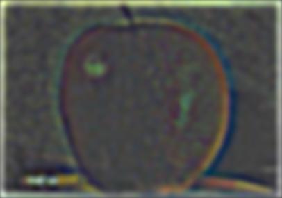
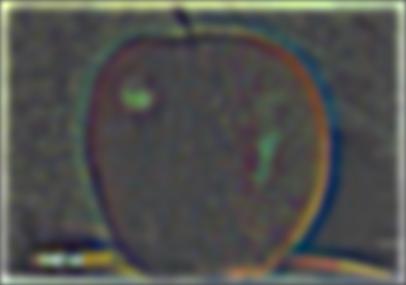
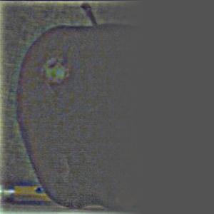
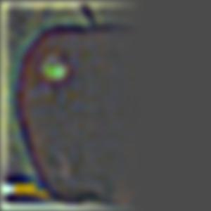
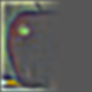
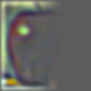
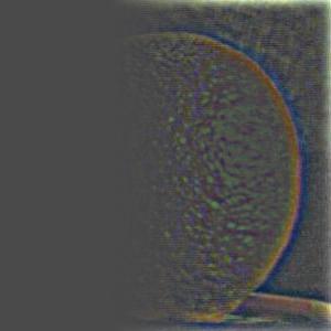
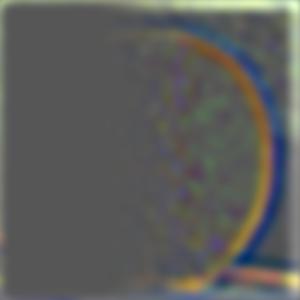
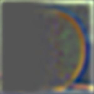
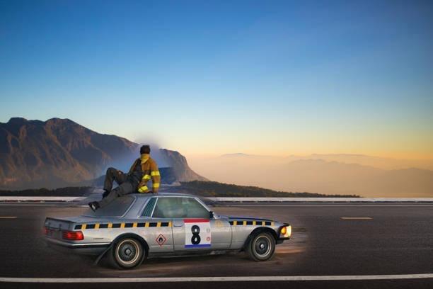
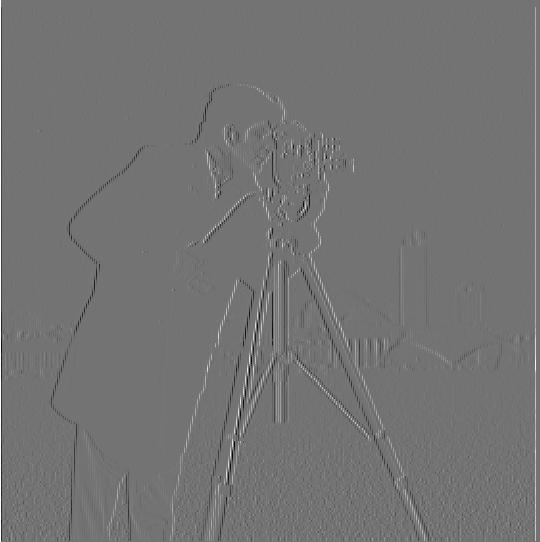
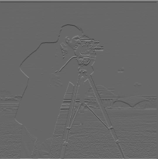
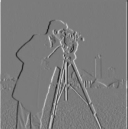
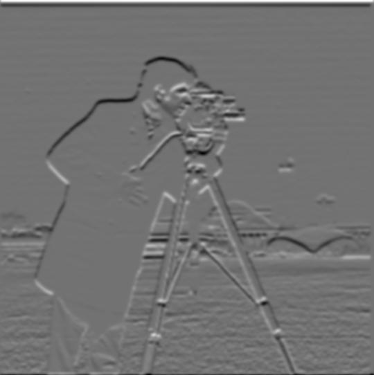
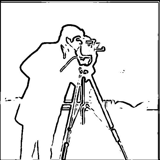
Here we convolve the image with two difference operators to look for edges. The respective operators are $D_x = \begin{bmatrix}1 & -1\\ \end{bmatrix}$ and $D_y = \begin{bmatrix}1 \\ -1\\ \end{bmatrix}$. We then take the magnitudes of the gradient values, where $(\nabla \text{im})_{ij} = \sqrt{(D_x * im)_{ij}^2 + (D_y * im)_{ij}^2}$. From here, we can define an arbitrary threshold to detect edges.

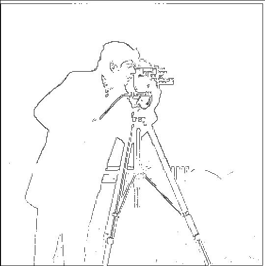
Image convolved with $D_x$	Image convolved with $D_y$	Image gradient magnitudes	Image edges (0.3 threshold)

Part 1.2. Derivative of Gaussian (DoG) Filter

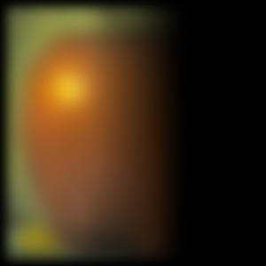
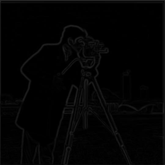
Here we do the same process except we pass the image through a Gaussian filter first. Instead of needing to perform two separate convolutions per direction, we can simply convolve the image with the filters $(GF * D_x)$ and $(GF * D_y)$.

Image convolved with $(GF * D_x)$	Image convolved with $(GF * D_y)$	Image gradient magnitudes	Image edges (0.05 threshold)

Part 2.1. Image Sharpening

In this part, we apply an unsharp mask filter to the image. Essentially, we Gaussian filter the image, and then subtract it from the original, producing an image with only high frequencies (and thus sharpened). We can parameterize the sharpening extent and also maintain the correctness of the output pixel values with the following formula: $$\text{unsharp}(\text{im}) = (1 + \alpha) \text{im} - \alpha GF(\text{im})$$ Using the properties of convolutions, we can thus create a single convolution that performs the unsharp mask filtering: $f = (1 + \alpha)I - \alpha GF$, where $I$ is the unit impulse.

Here is the unsharp mask filter on a couple custom images:

Original Image	Gaussian Filtered Image	Resharpened ($\alpha$ = 1.1)

Part 2.2. Hybrid Images

To create hybrid images, we low-pass filter one image and high-pass filter the other, and then add them together. As such, two different images can be seen at different distances. This portion took a decent amount of tuning, as the parameters were dependent on the images themselves.

The high pass filter used was the unsharp mask filter: $HP_\alpha(\text{im}) = \text{im} - \alpha GF(\text{im})$, and the low pass was an amplified Gaussian filter, $LP_\beta(\text{im}) = \beta GF(\text{im})$.

Image1 (High passed)	Image2 (Low passed)	Merged Image

Here are the results on some custom images

Image1 (High passed)	Image2 (Low passed)	Merged Image

We can also perform frequency analysis on these images:

Image1 Initial Frequencies	High-passed Image1 Frequencies	Image2 Initial Frequencies	Low-passed Image1 Frequencies	Merged Frequencies

Bells and Whistles

I tried four variants of creating the hybrid images: using color from both images, using one colored image and one greyscaled image, and using greyscale for both. It seems like only coloring the high-passed image or using the doubly-greyscaled image is the most ideal. However, this could also be due to the particular configurations of the pictures that I tried.

Double Color	Only Color High-pass Image	Only Color Low-pass Image	Double Greyscale

Part 2.3. Multi-resolution Blending and the Oraple journey

Below we show the Gaussian and Laplacian stacks of the oraple, as well as the masked Laplacians of the apple and orange images respectively:

Part 2.4. Multiresolution Blending

Here are some fun blending examples that I did:

Aligned Image 1	Aligned Image 2	Mask	Blended

Bells and Whistles

All of the blended images were done with color.