CS194-26 FA21 Project 2: Fun with Filters and Frequencies!

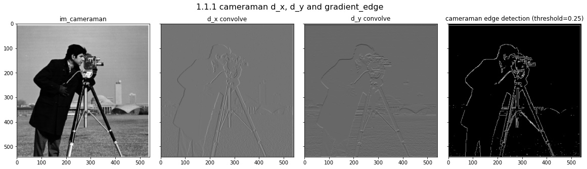
I start with initial cameraman and convolve with finite difference filters for x and y directions separately. Then take both results, square each pixel value, and then take the square root of the sum to compute the magnitude of the edge gradient. I then threshold the edge magnitude image to create a binary edge image. Results somewhat noisy.

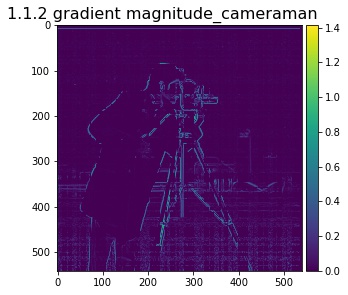
Magnitude of the gradients computed as described above before we compute the threshold.

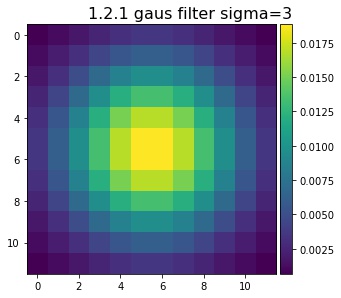
Gaus filter we are going to use to blur images. The sum of all values is 1.

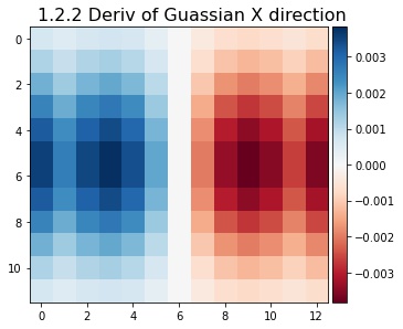
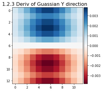
Convolve the finite difference filter with the Gaus in the x direction to combine the operations.

Do the same for the y direction.

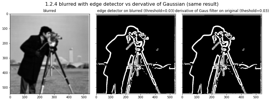
To reduce noise in our edge detection I remove high frequencies by convolving the image with a Guassian (low pass filter). We can then run the same edge detection procedure descrived in 1.1.1 and we get a cleaned up edge dection image. To skip having to first blur then convolve with finite difference filters, we can just convolve with finite difference filter with the Gaus (1.2.2 and 1.2.3) and then apply this new mask to the image. Note that the results in the second two images are exactly the same as we would expect. Question: what differences to you see (after blurring)? Answer: once the image is blurred the edges detected are much thicker. This makes sense because blurring creates continuous and smoother areas of change in the image. Also there is much less noise which makes sense because we have reduced high frequency compoents.

Low pass filter the Taj by convolving with the Gaussian. Then subtract this blurred image from the original (scaled by some coefficient) and we get an image with the high frequencies increased.

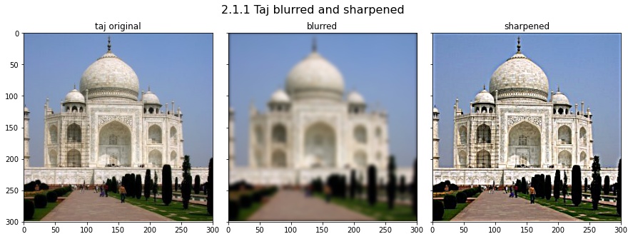
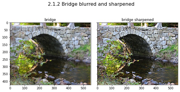
The sharpening procedure can be done in one step by subtracting a guas kernel from the identify kernel to make an unsharp mask filter. Now we just convolve with the unsharp mask filter to easily sharpen. Results are shown below.

The input image here has top half unsharpened and then the bottom half already sharpened. I apply my sharpenening across this whole image. Notice the changes at the edges of the lines!

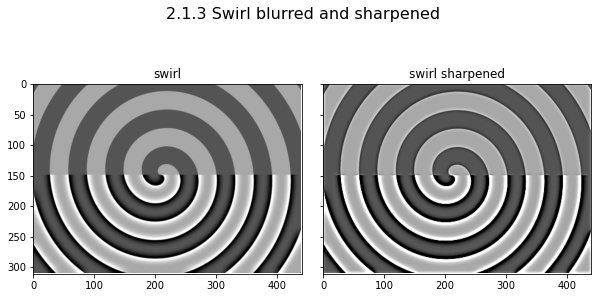
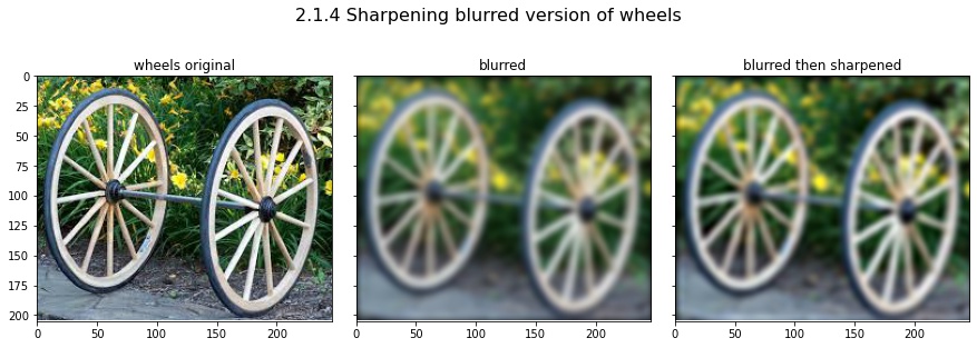
If we blur and then try and sharpen the blurred image the resulting image is still pretty blurry. This is because the blurred image already has the high frequency components removed and the information about those high frequencies are lost by blurring and are not recoverable.

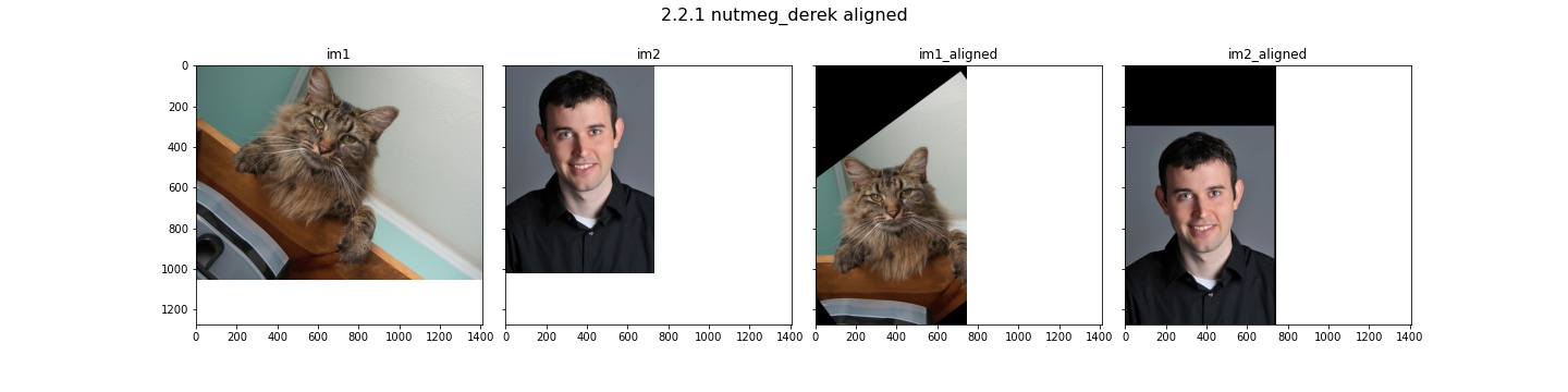
Now I implement the hybrid images algorithm. The first step in making hybrid images is aligning two input images. Here is the first images aligned. I picked the eyes to align.

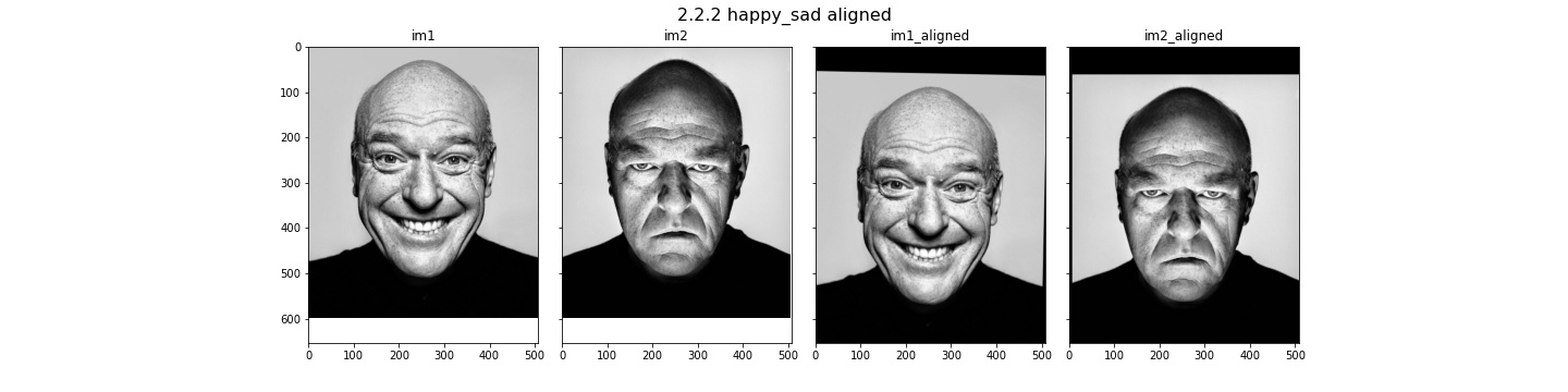
Here I pick the top and bottom of the head to align.

Here I pick the top left and bottom right corners to align.

Here I pick the eyes to align.

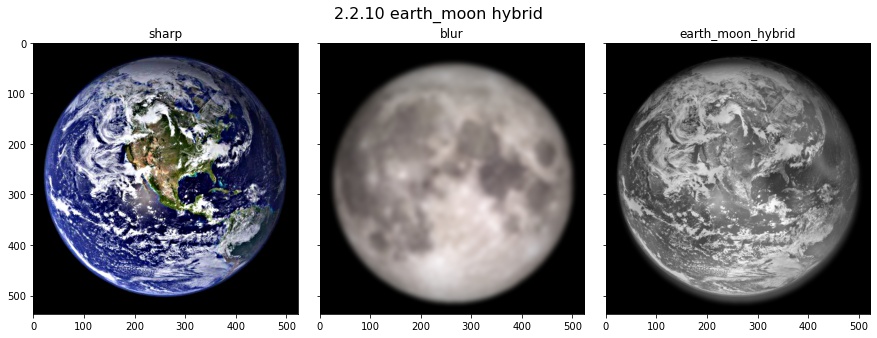
I pick the top and bottom of the planet/moon to align.

Now that images are aligned we can to the hyrid image algorithm. We sharpen the first image an then blur the second image and then average the two results together to get the hybrid image. The idea is that humans are good at seeing sharp images (high frequencies) up close and see the burred (low frequency) images farther away. So if you are close you see a cat and if you are farther you see the person.

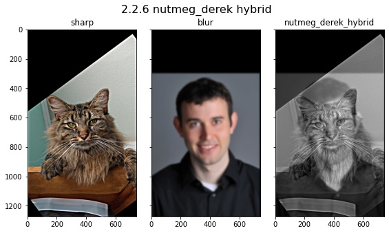
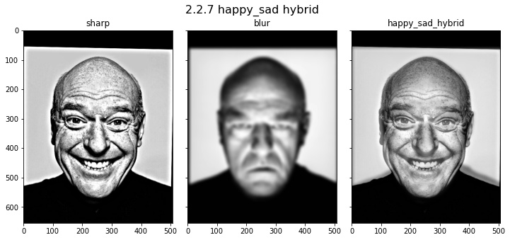
Here I tried a facial expression hybrid. It did not work that well because the teeth in the smiling picture are still very clear in the resulting image even at far distances, so it always seems like he is smiling.

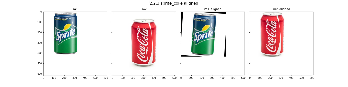
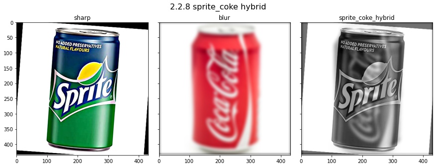
Here is another failure case. The text on the cans do not align all that well so even the text on the coke can is visible from far away, which breaks the illusion. Also the alignment was not great.

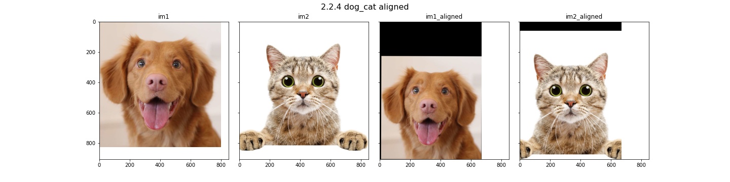
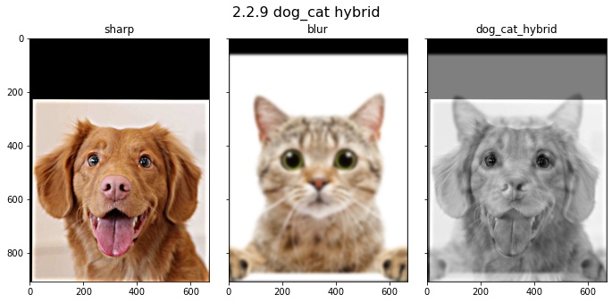
Here is the best result. The dog is clearly visible up close and the cat is visible farther away. This worked well since the face shape was similar and features aligned.

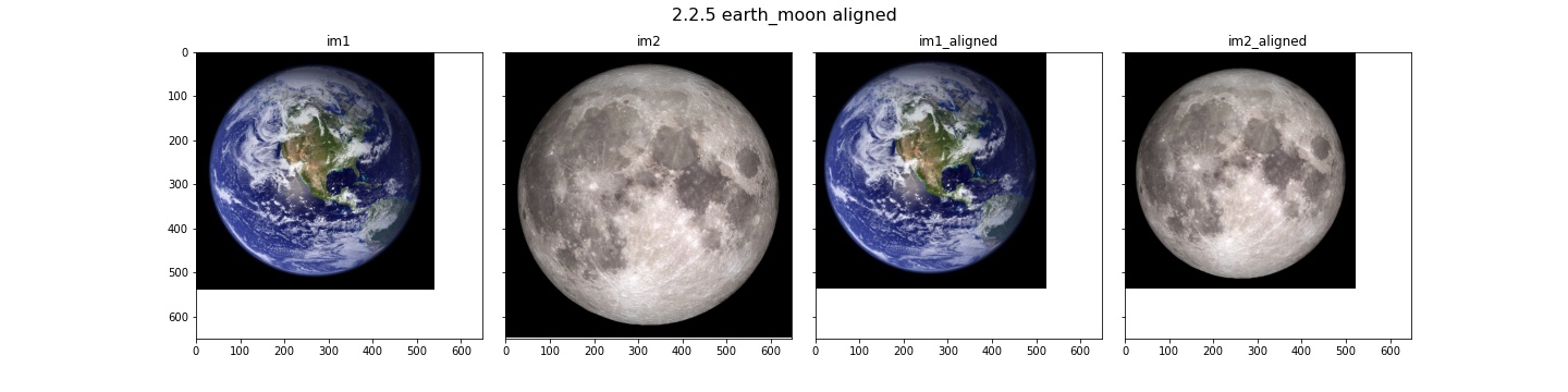
Here is another failure case. The clouds on the hybrid image break the illusion.

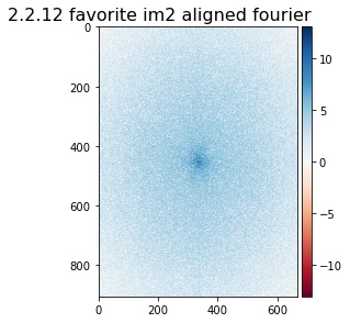
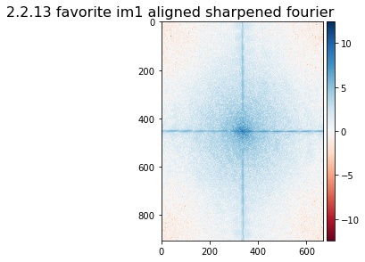
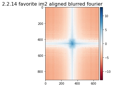
Doing Fourier analysis is interesting here since we are playing with the frequencies of the input images. The Fourier transforms (FT) shown here are of the images used in 2.2.9 (im1=dog(sharpened) and im2=cat(blurred)). Here is the FT of the dog after alignment.

Here is the FT of the cat after alignment.

FT of the dog after sharpening. Comparison to 2.2.11 will show that values farther from the origin have increased indicating a boost in high frequency.

Here is the FT of the cat after blurring. Comparison to 2.2.12 shows that high frequency components have dropped significantly.

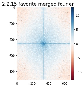
After merging the images we get the following FT. It looks like this FT is a combination of the past two, which is what we would expect since we averaged the two inputs.

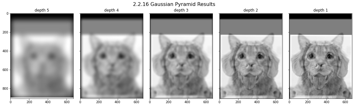
Potential bell and whistle: I implemented Guassian pyramid and applied it to the hybrid image of the dog and cat. During the pyramid the image gets repeatedly blurred then downscaled. Here I scale the iamges back up just so they can be the same size for visual comparison.

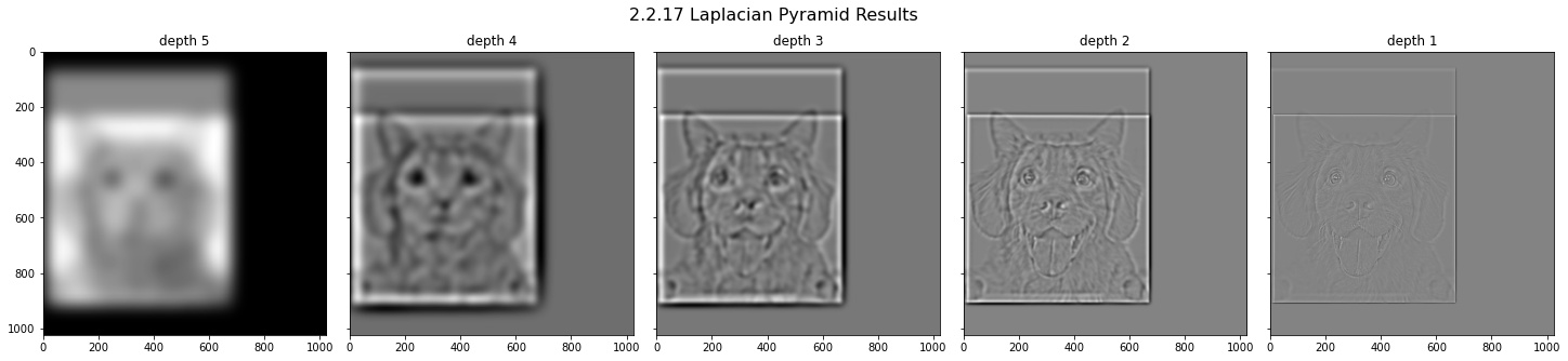
Potential bell and whistle: Also not sure if this was required, but here are the Laplacian pyramid results. The entries in this pyramid can be constructed by subtracting adjacent layers of the Gaussian pyramid (after scaling back up the image at the lower depth). As before I scale images to same size here just for display purposes. The original image can be reconstructed by scaling and then adding all these layers back together.

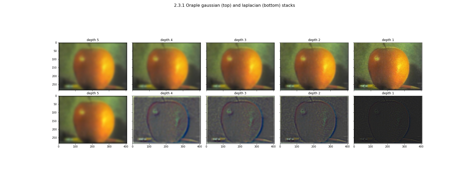
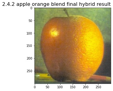
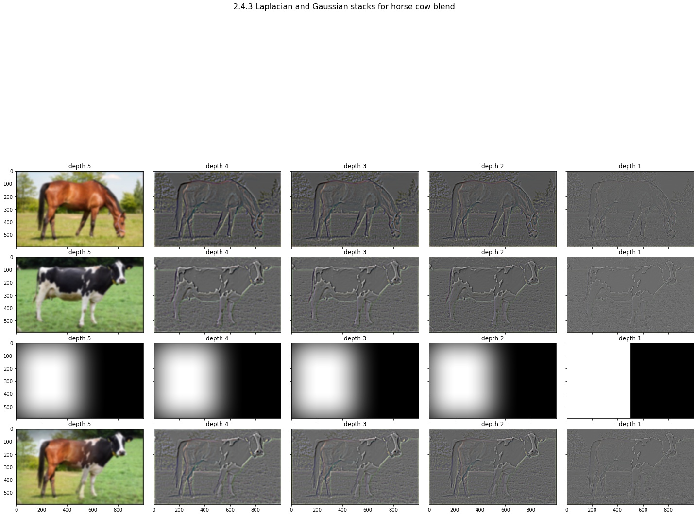
I then implemented the Guassian and Laplacian stack algorithms. These are very similar to the pyramid algorithms except we do not scale the images down at each level. I applied these algorithms to the Oraple as shown below. To see the visualization with the mask applied to each corresponding layer of the Laplacian stack, please see the images further below in section 2.4.

Now for multi resolution blending! The main idea is we can achieve a nice transition between two images by blending at different frequency bands. The laplacian stack helps us get a different band frequency in the input image at each of the different layers. So we first apply Laplacian stacks to two input images we want to blend (row 1 and row 2). Next we apply a Guassian stack to the step function (row 3). The row 3 images represent a spline which is the edge where we transition between the images. Next, for each depth (column), we blend the correspoding frequency bands from the two input images by weighting the pixels by the spline image (row 3). We do this weighting operation for each depth to produce row 4. Note that since the spline image has more blur at deeper levels we are combining lower frequency bands of the inital images across a greater area and higher frequency bands of the intial images across a small area. This makes sense as low frequency components spread farther across an image. Note that I scaled the intensity values for the images that were outside of the 0-1 range back to the 0-1 range in order to visualize them in the images presented here. The scaling was only done for visualization and the actual algorithm operates on the raw versions.

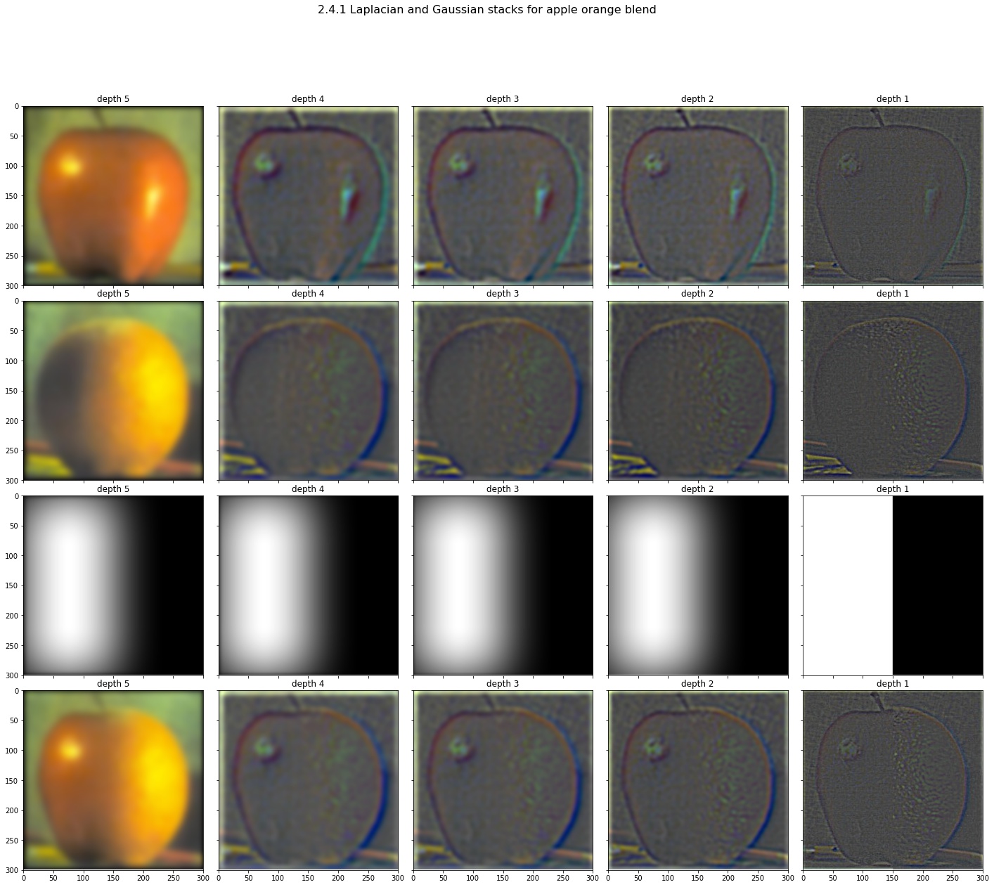
Now we just need to sum together the the entries in the final rows to combine all the blended frequency bands to construct our final results pictured below!

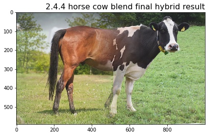
Here is the same procedure for a horse and a cow.

And the result! The slight misalignment at the top of the cow with the horse makes the illusion less strong, but the blending still did work somewhat.

Instead of using a step mask we can use a more interesting mask such as this circle cutout. The final result is pretty good, but could be improved by having an eye picture that actually contained more of the face and did not have a sharp edge to the white background that ends up being present in the final result.

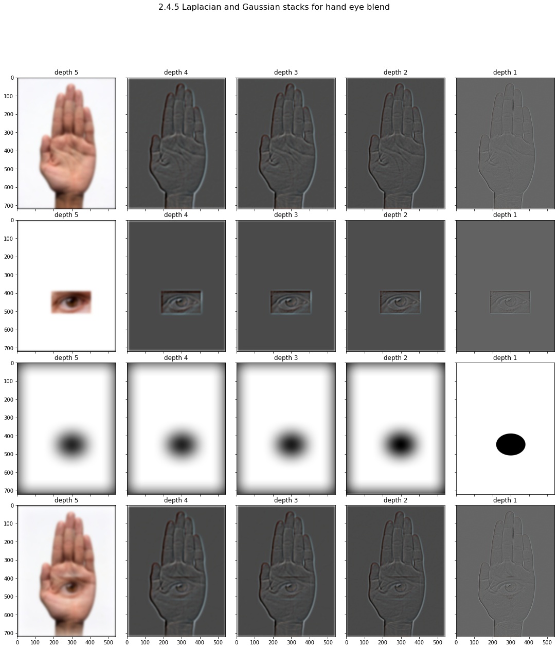
The final hand eye merge result! Bell and Whistle: all these multiresolution bending images support color in the output!