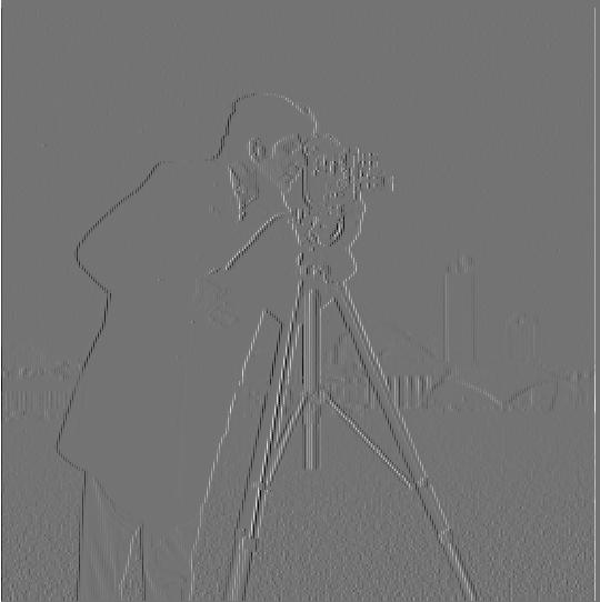
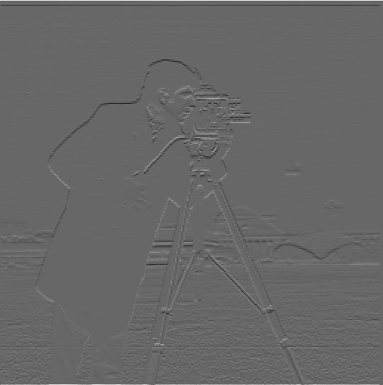
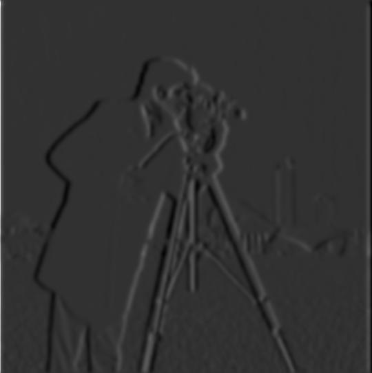
For this part of the project, we want to compute the gradient magnitude. In order to do this, we first define finite difference filters in the x and y directions: D_x = [1, -1] and D_y = [1, -1]^T. We then convolve (scipy.signal.convolve2d) these filters with an image to get the gradient of an image in the x-direction, and the gradient of an image in the y-direction. Then, in order to get the gradient magnitude, we compute by doing √(gradient_x^2 + gradient_y^2).
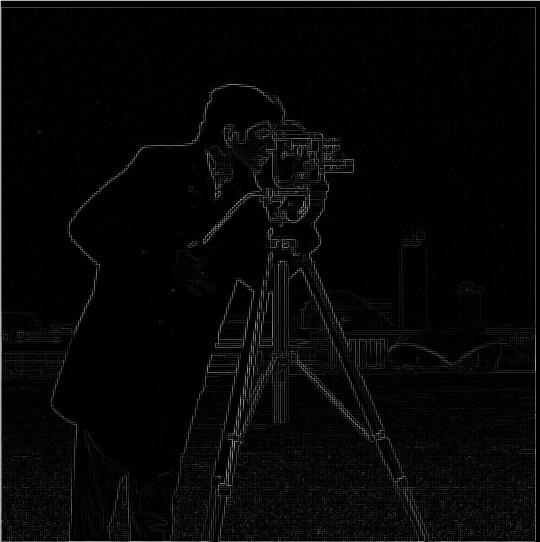
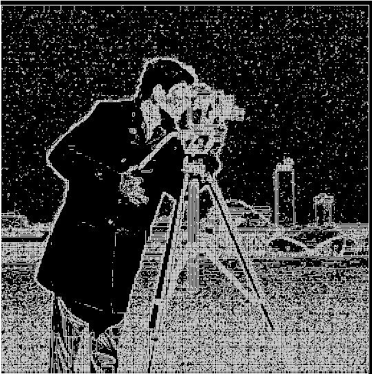
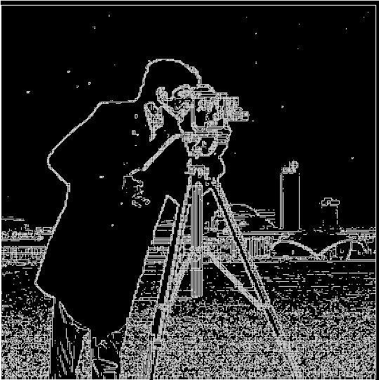
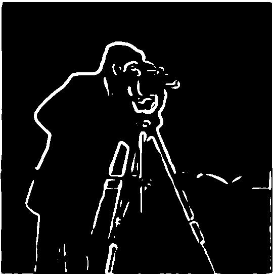
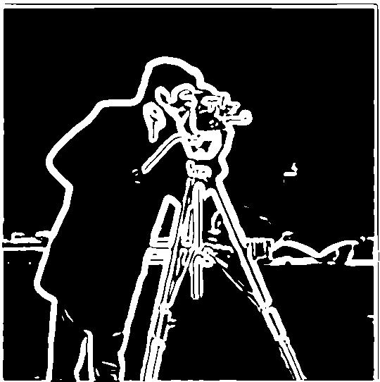
Next, after binarizing the image using a threshold, the gradient magnitude will show all the edges of an image. Below are some examples of what edges show with different thresholds:
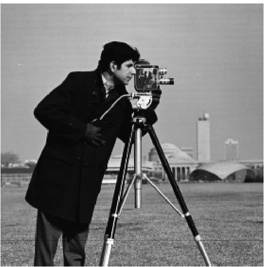
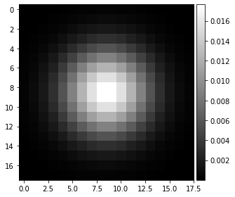
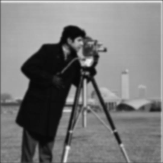
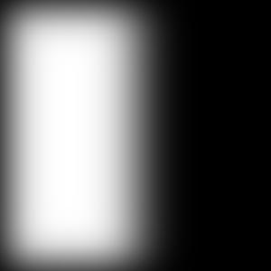
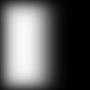
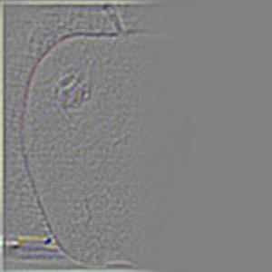
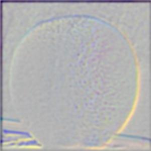
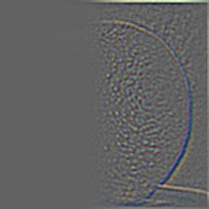
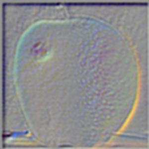
Sometimes the above process is not great because edges can be noisy. We can address this by running a low-pass filter over the image using a Gaussian kernel to blur some edges. To create a Gaussian blur filter, we first create a 1-D kernel (cv2.getGaussianKernel), then matrix-multiply with itself to get a 2-D matrix. We can manipulate its size and sigma to strengthen or weaken the blurring effect. With this Gaussian filter, we convolve it with the cameraman image. Below we have the original image, Gaussian filter (size=18, sigma=3), and blurred image:
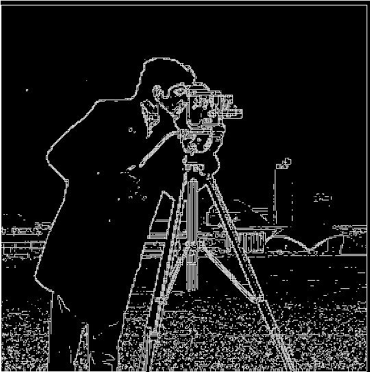
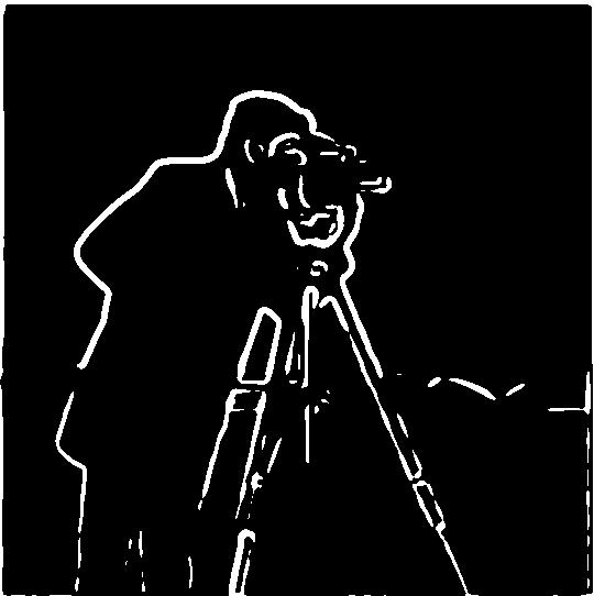
Now, let's see the results of repeating the above process again, but on the blurred_cameraman image:
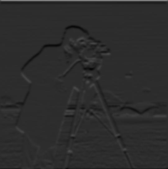

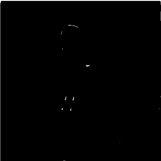
It is quite clear here that the blurring has made edges less noisy, and comparing 1.1 and 1.2, less edges are seen in the gradient magnitude image of the blurred original image.
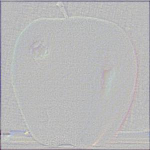
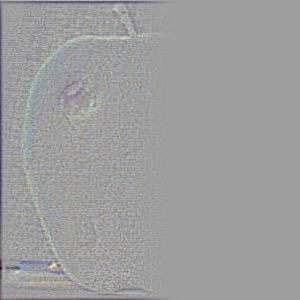
We can also try a different method: instead of convolving the Gaussian filter with the image and then calculating the partial derivatives, we can convolve the Gaussian with the finite difference operators and get the derivative of gaussian (DoG) filters.
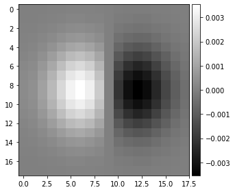
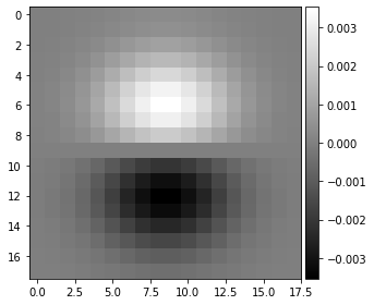
Answering the question in 1.2: When comparing the gradient magnitudes from 1.1 and 1.2, we see that the 1.2 edge detection is more obvious.
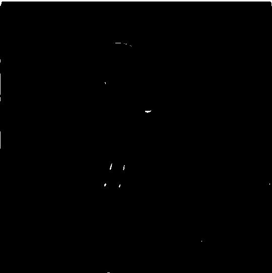
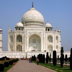
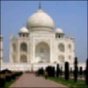
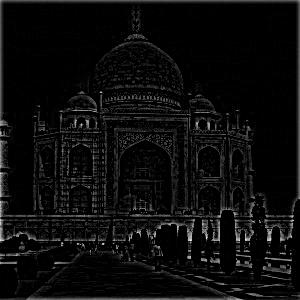
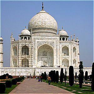
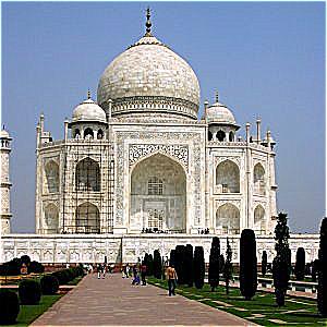
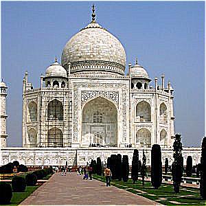
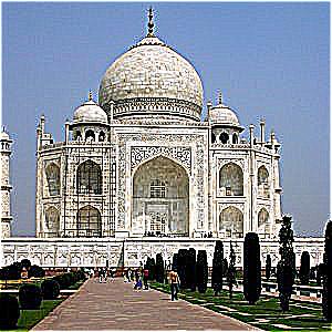
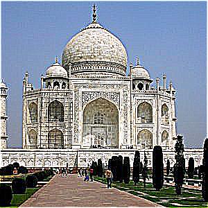
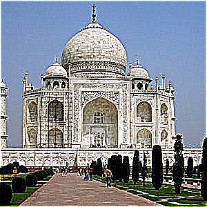
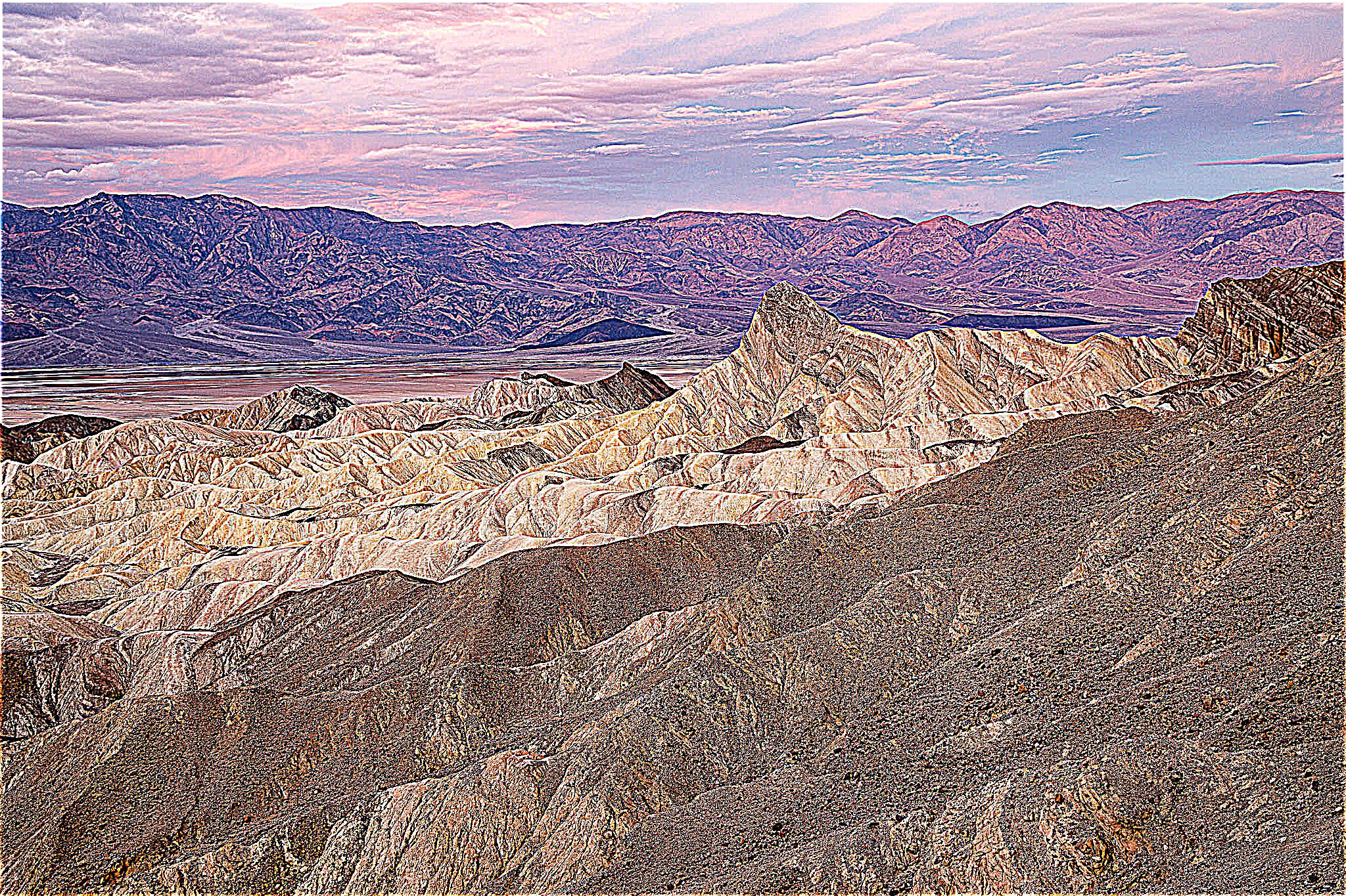
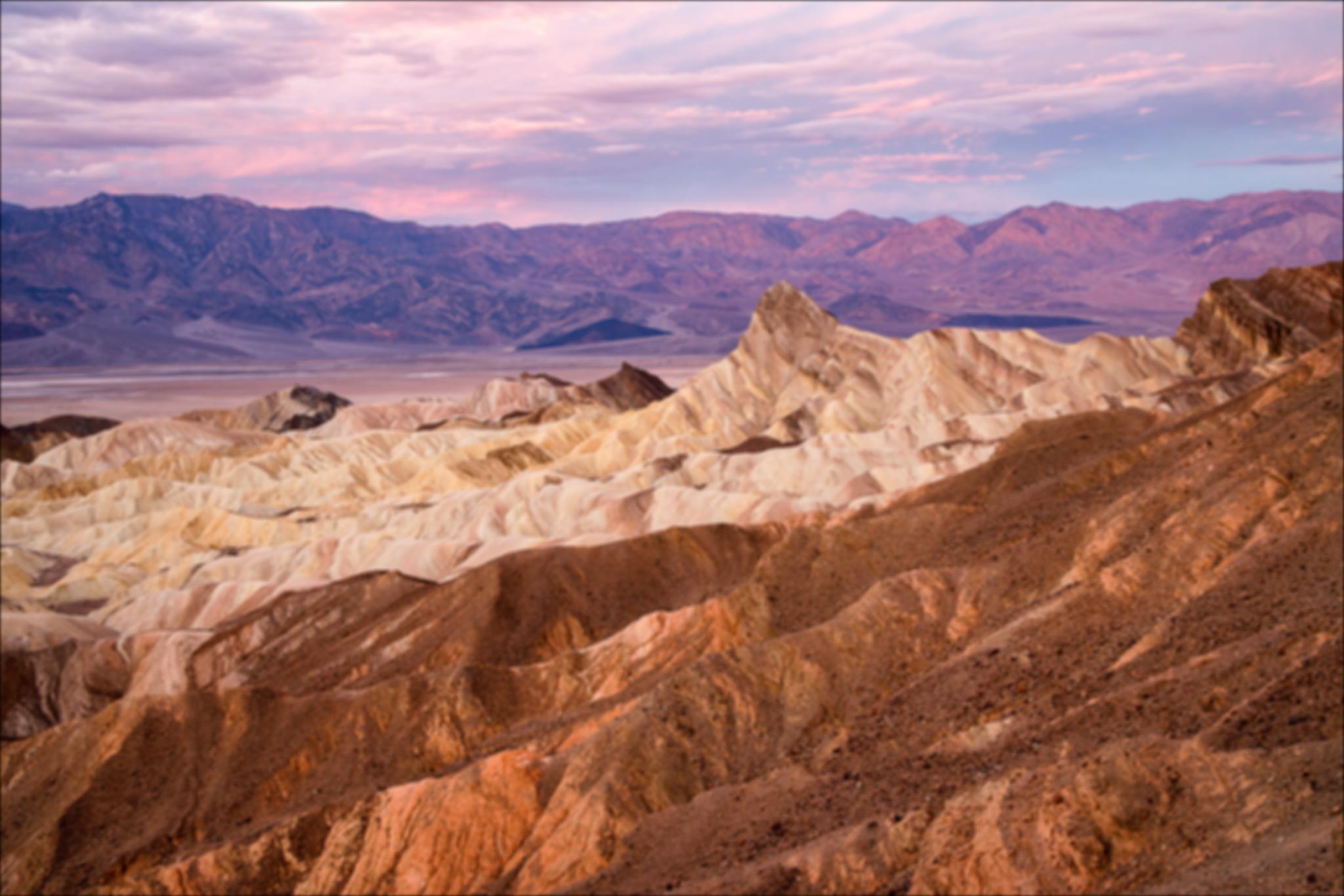
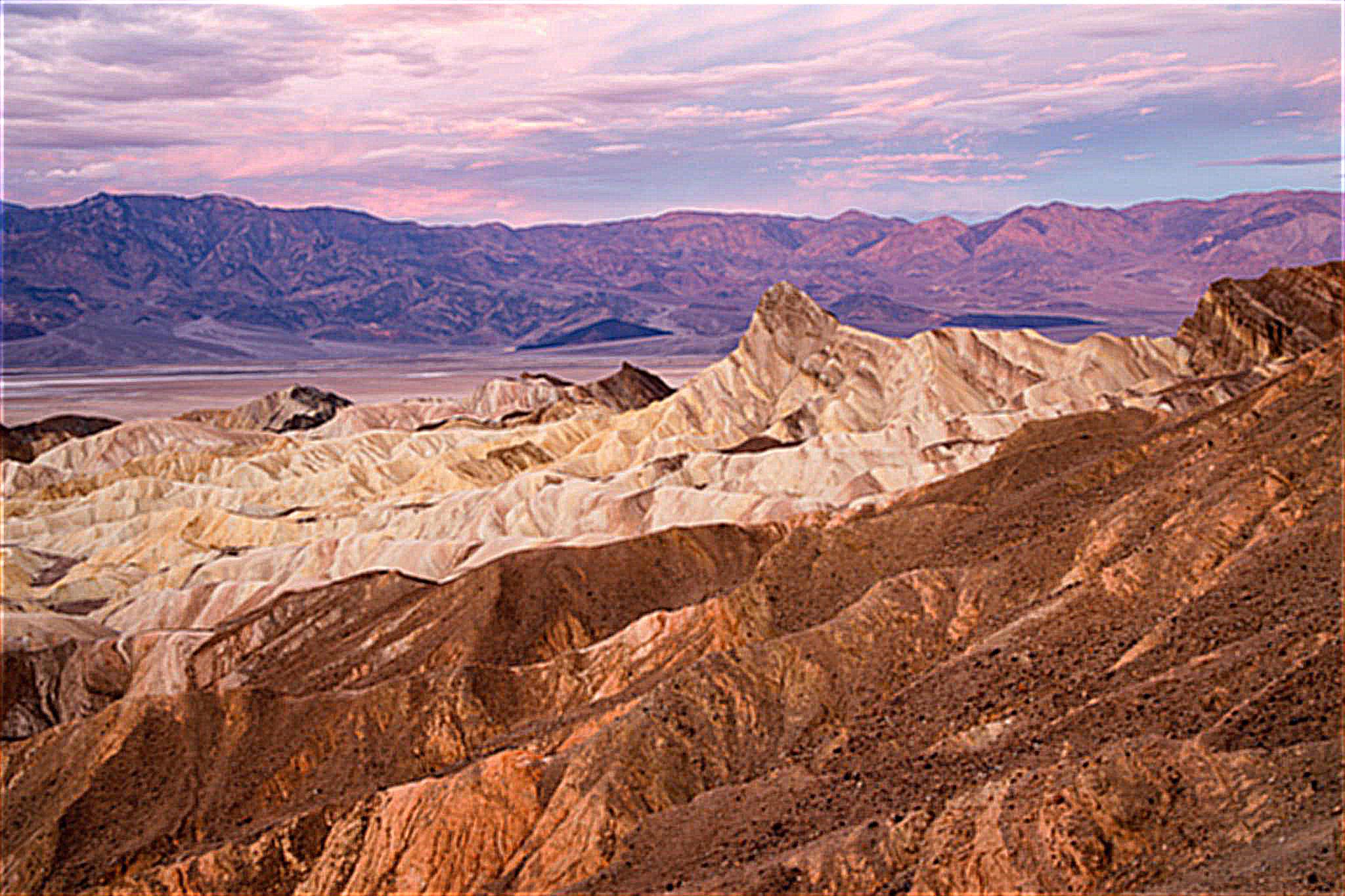
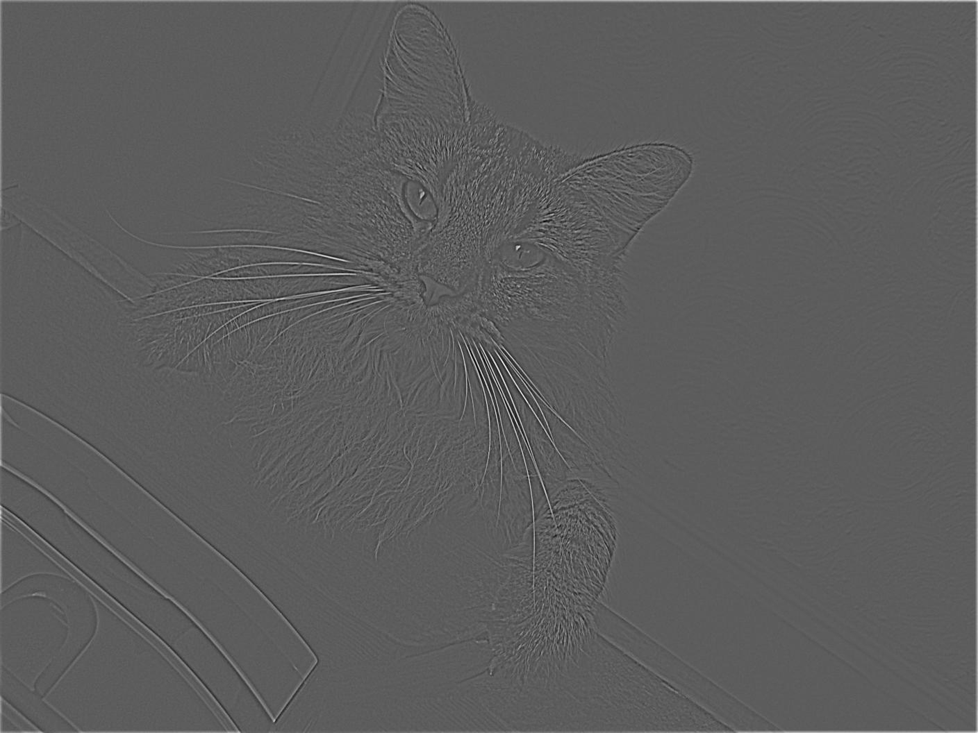
To sharpen images, we highlight the high frequencies of the image. In order to get the high frequencies, we do original image - blurred_image = high_frequncies. This works because the Gaussian filter acts as a low-pass filter and retains the low frequencies. Below are the original Taj, blurred (Gaussian size=9, sigma=3), and high frequency (scaled by 10 and clipped to be between 0 and 255):
Now that we have our high frequencies, we can sharpen images following: sharpened_image = original_image + α * (original_image - blurred_image), where α is the scalar factor to indicate how much high frequency to add. Below are examples of sharpening with α from 1 to 10:


I've also sharpened two other images as examples. Below are the results with α = 1, 5, 10:
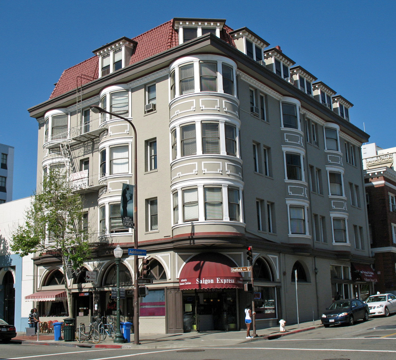
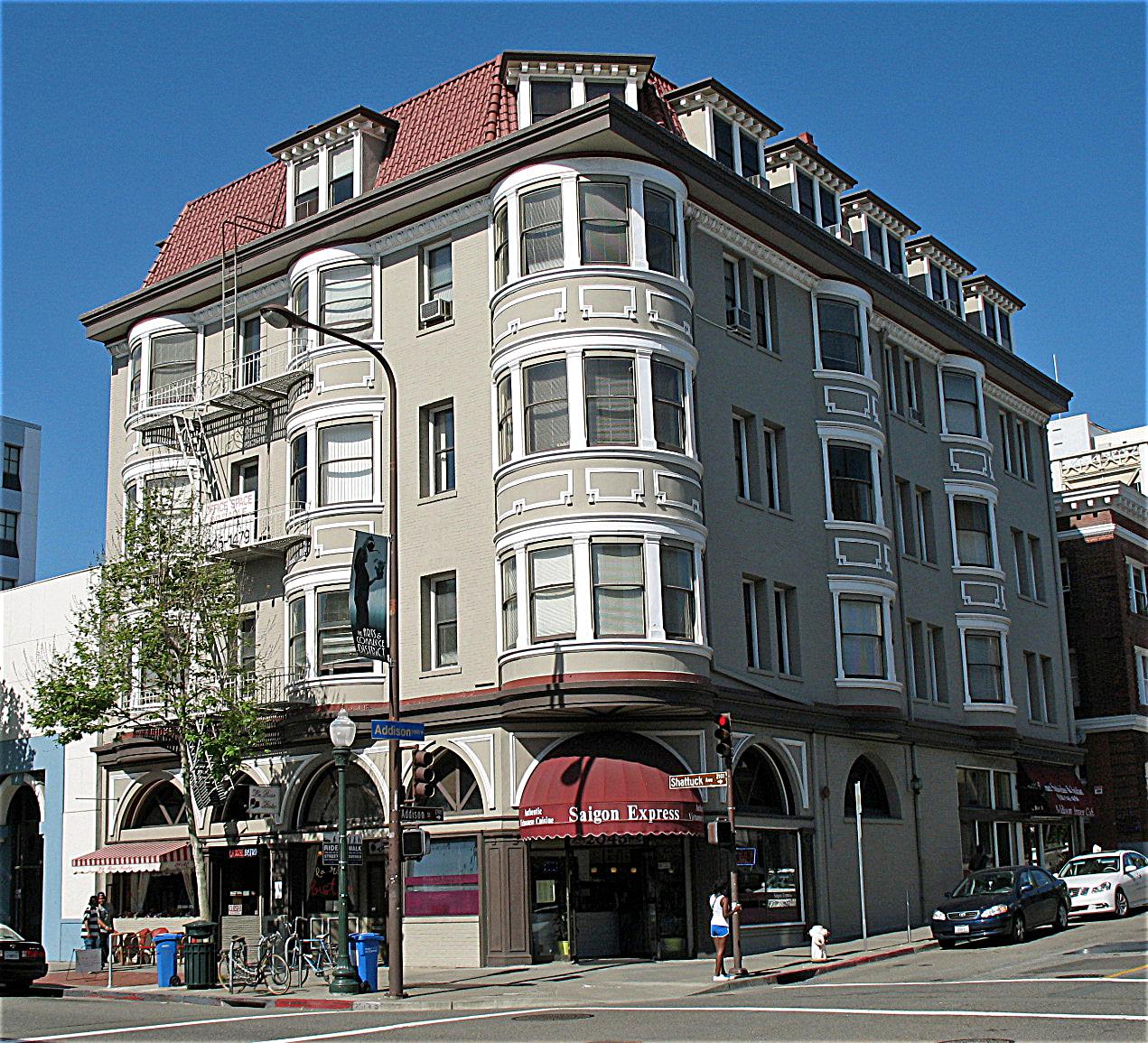

As a comparison to the sharpening process, let's blur a sharp image, then try to sharpen it again. Below are the original image, blurred (Gaussian size=9, sigma=3), and sharpened on blurred image:


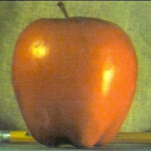
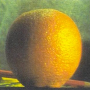
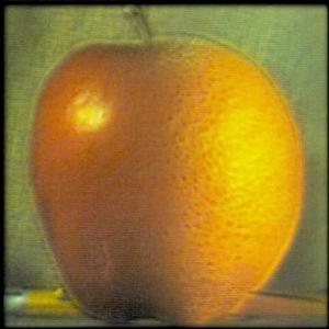
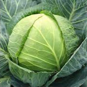
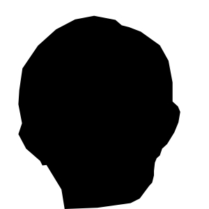
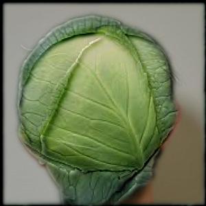
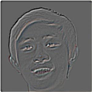
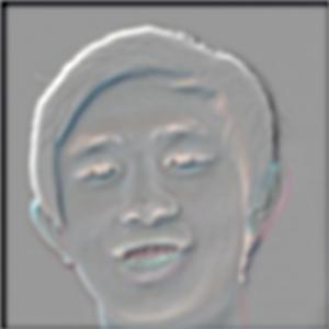
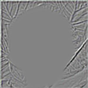
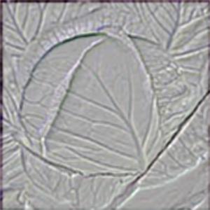
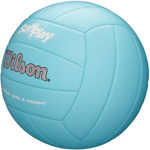
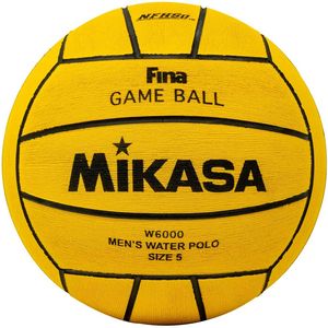
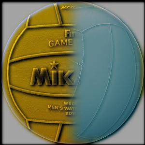
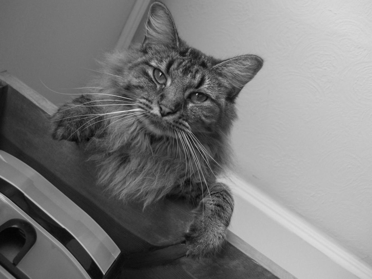
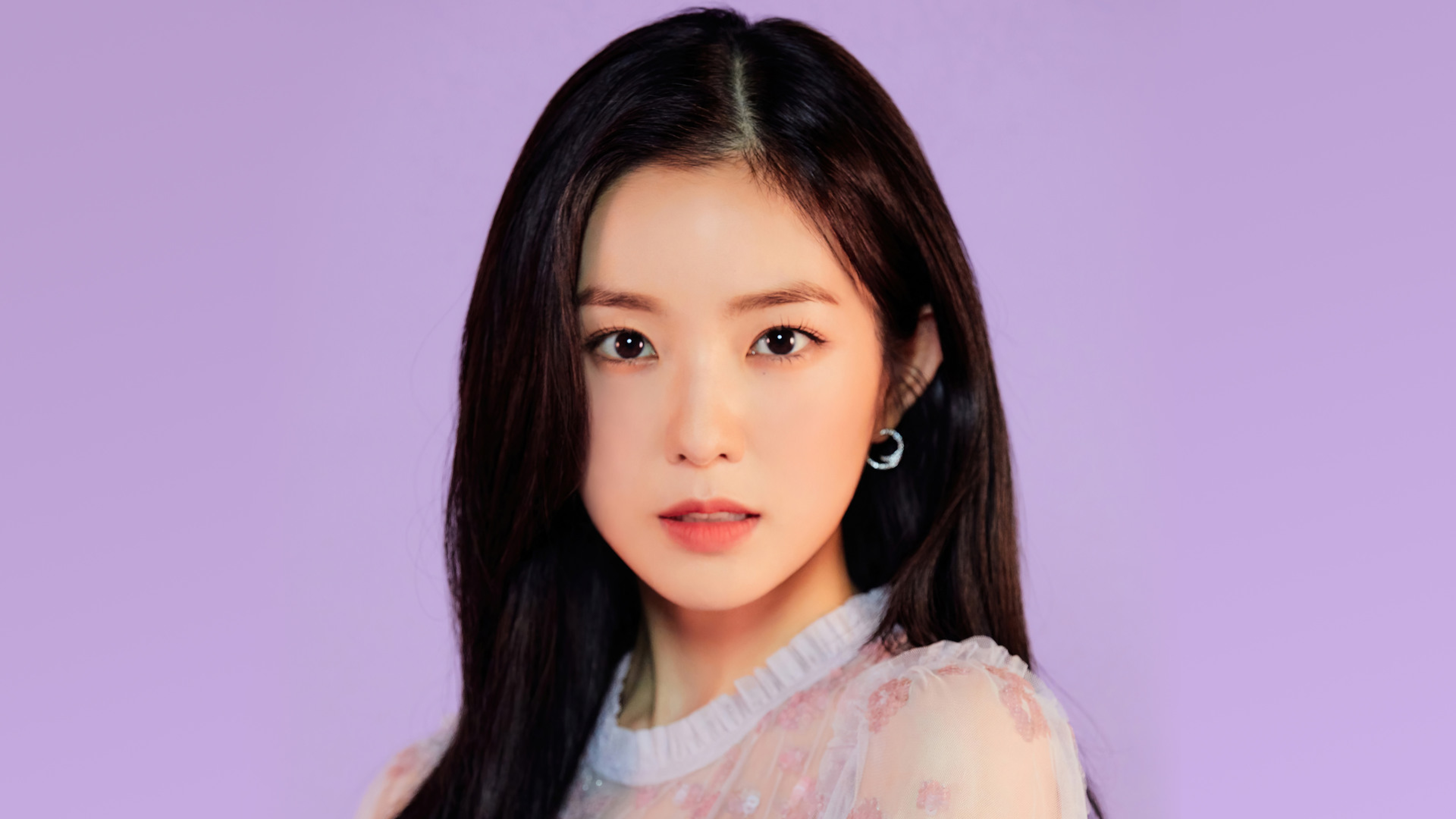
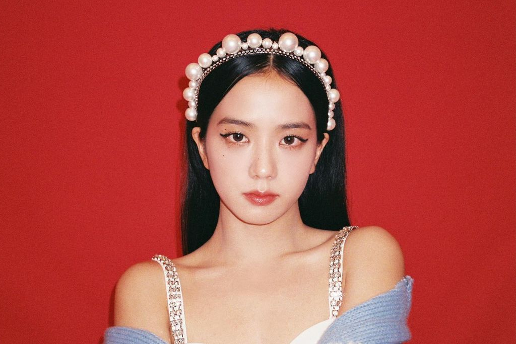
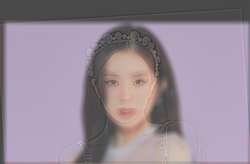
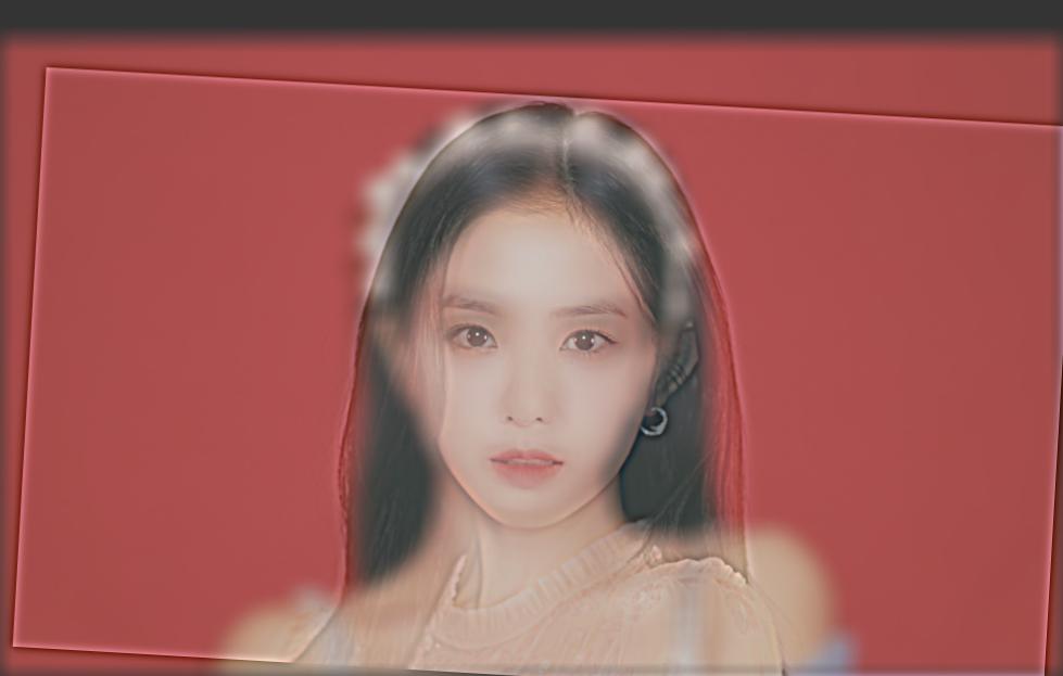
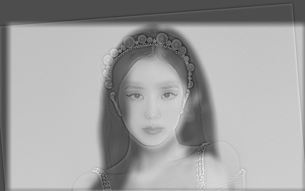
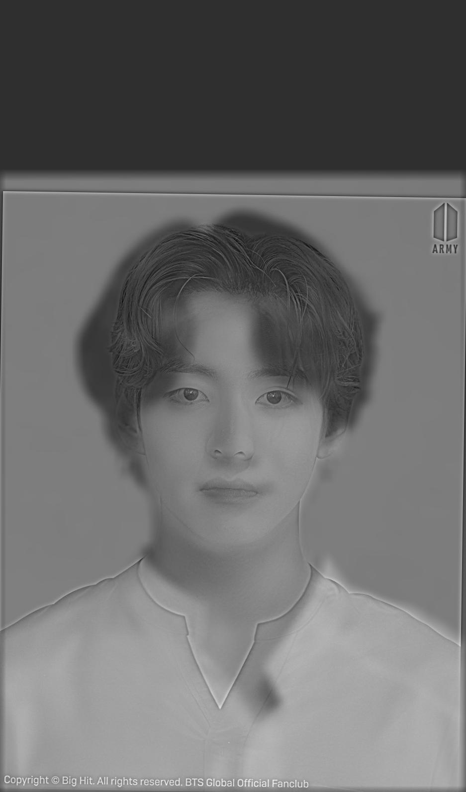
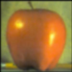
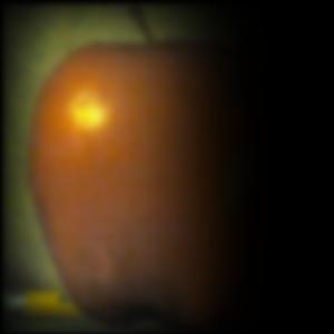
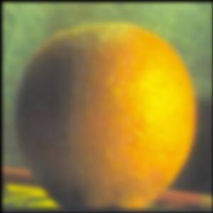
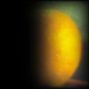
With our knowledge of low and high frequencies, we can try to combine the low frequencies of one image and the high frequencies of another image to create a hybrid image. The formula we followed was hybrid = blur(image1) + image2 - blur(image2). Let's take a look at the frequency domains of the images:

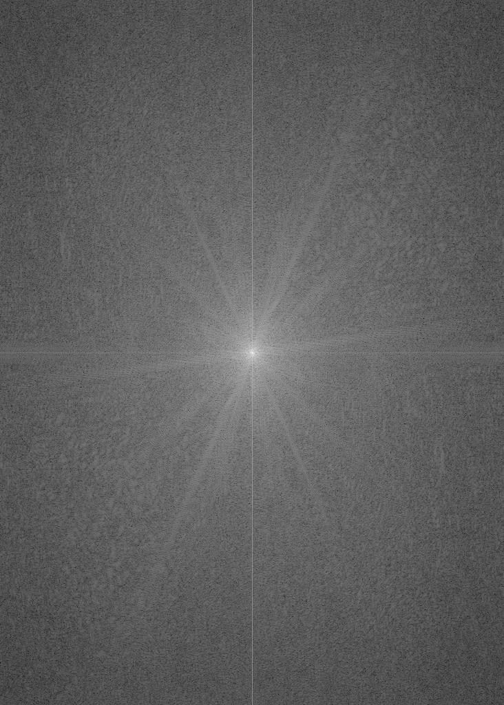
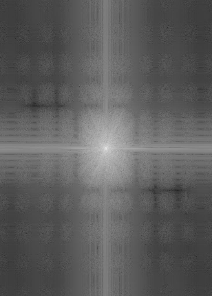
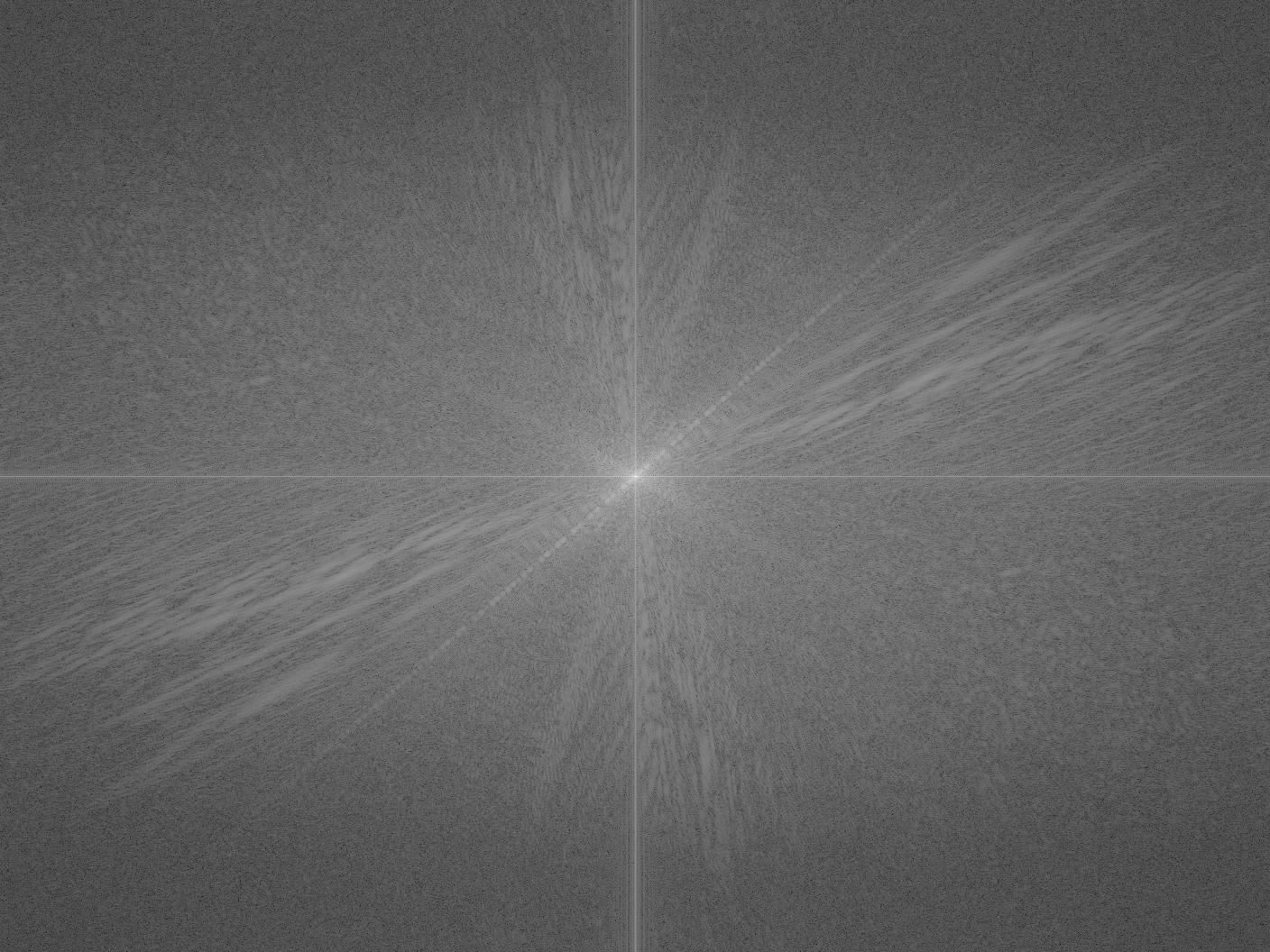

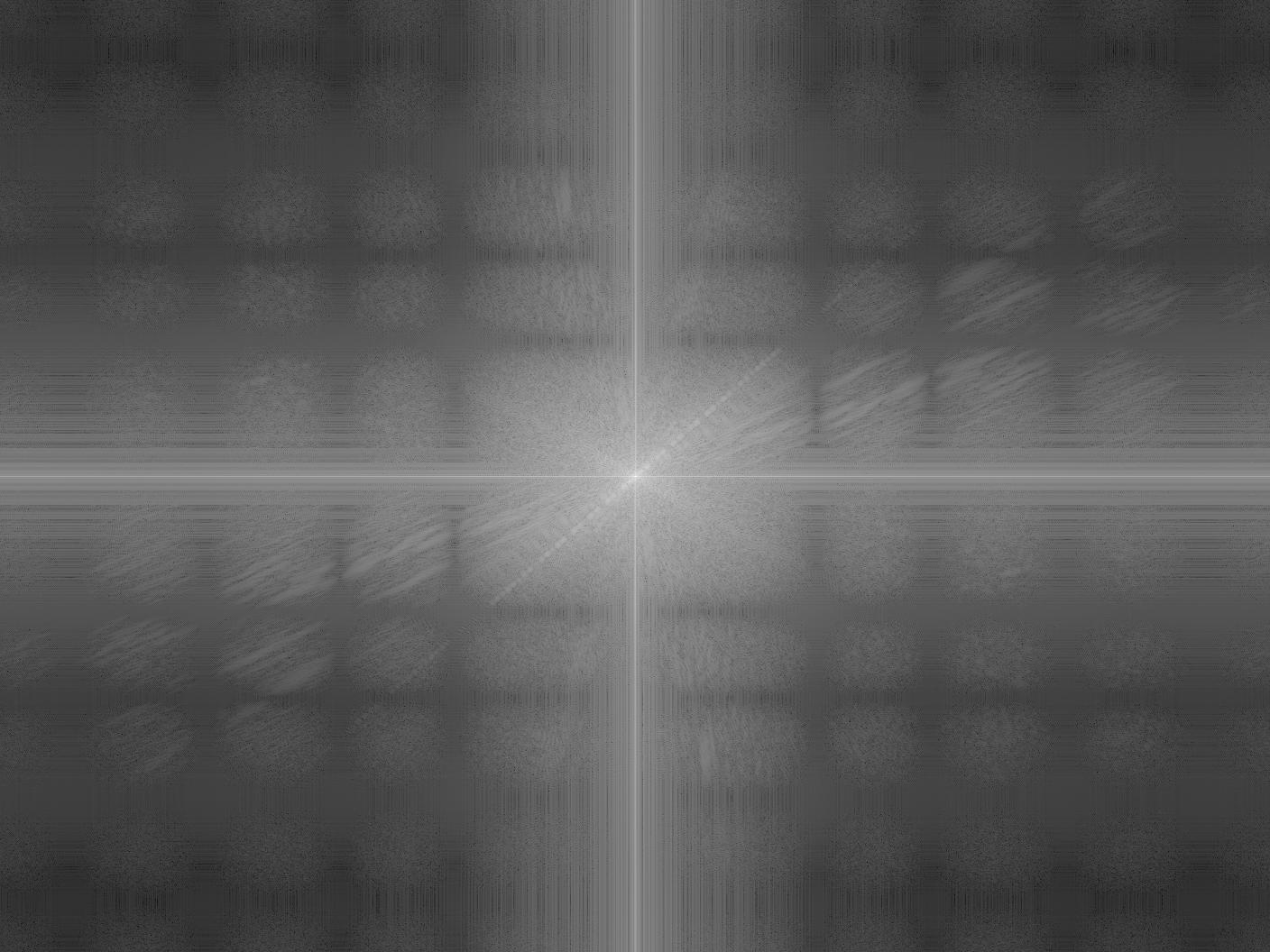
We can see from the frequency domains generated that with the Gaussian blur filter, only the low frequencies remain, and the opposite for the high frequency image.
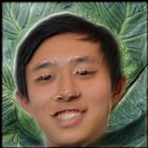
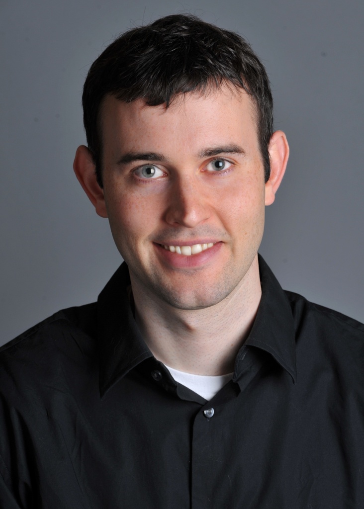
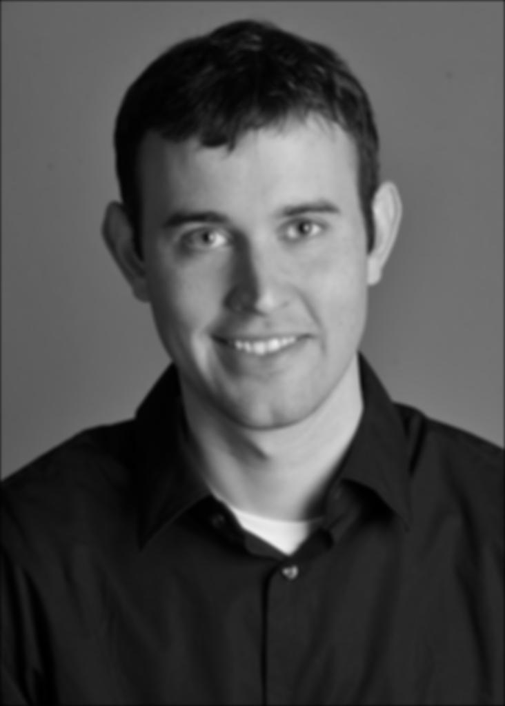
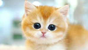
Now let's actually merge Derek and Nutmeg:
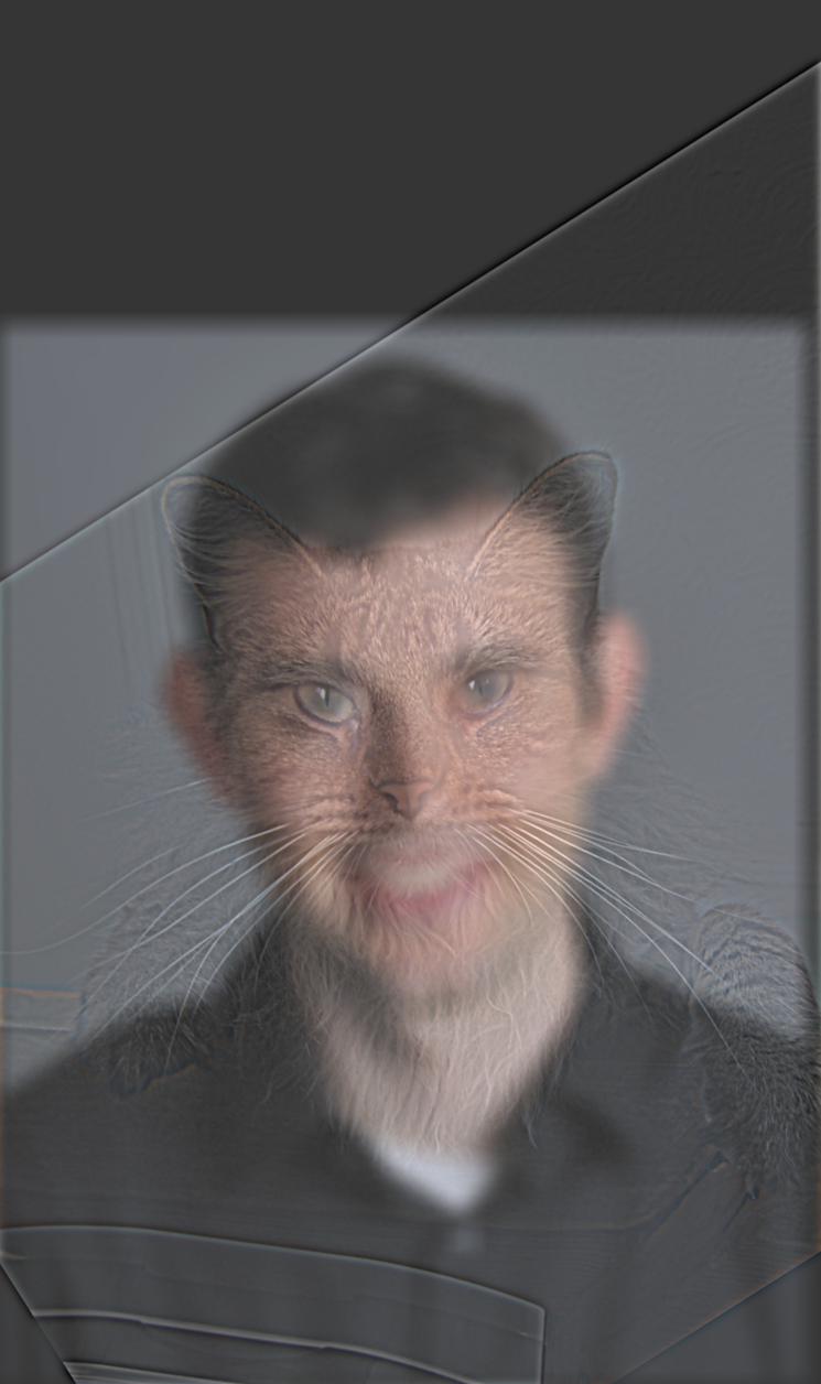
Color merging is done by computing reach RGB channel separately, then stacking together again.
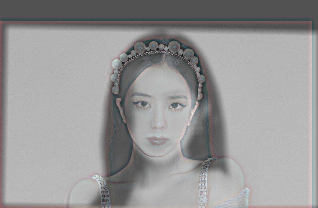
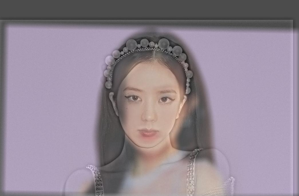
It seems that having the low-pass image be in color makes the image easier to see since it composes the majority of the background. Ultimately, having both the high and low frequency images be in color seemed to have the most cohesive result.


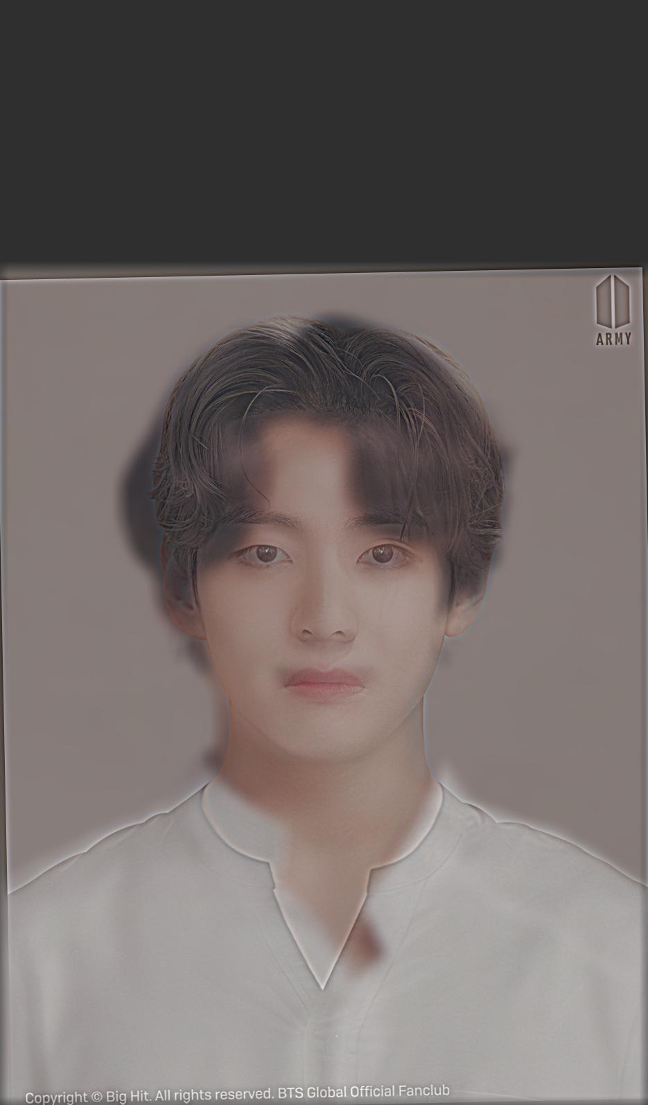
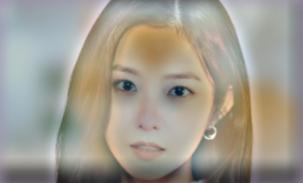
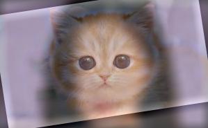
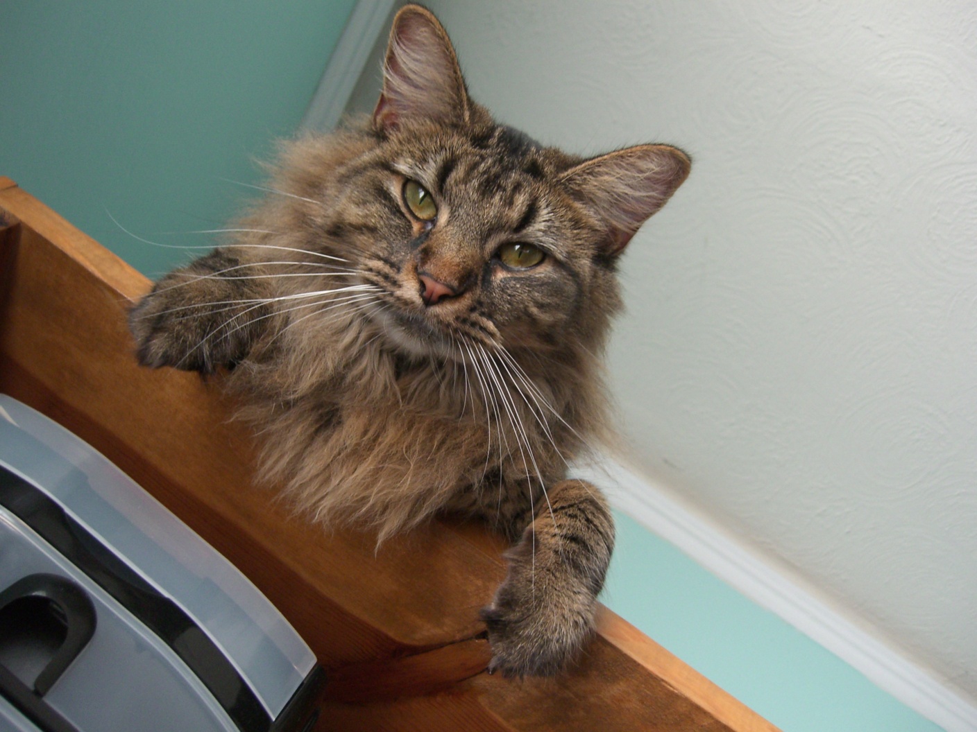
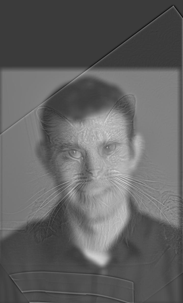
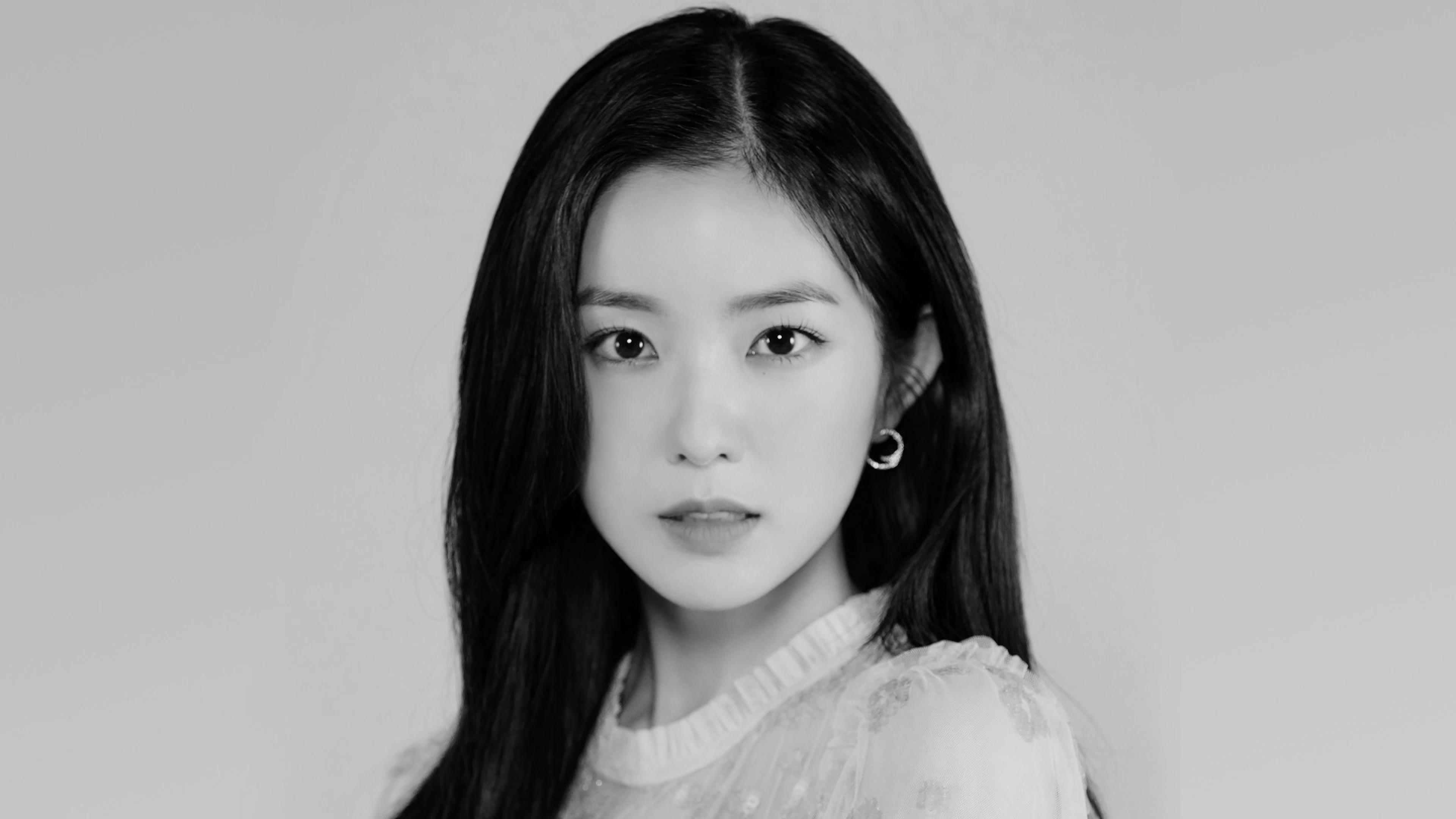
From this failure, we see that there are image scaling and placement issues. Because the cat face is much larger than Irene's, the hyrbrid merge does not align as well. If I had more time to work on this, I would try to have a dynamic rescaling to better align images.
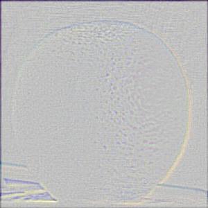
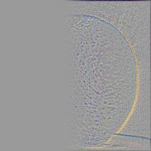
Now we want to blend images together along an image spine. This is done by using a mask applied to the two images in order to select which areas to merge into the final image. To do this, we first create Gaussian and Laplacian stacks of both images.
A Gaussian stack is iteratively convolving the Gaussian filter onto the previous image: gaussian_stack[i] = blur(gaussian_stack[i-1]), where blur() convolved the Gaussian filter with the image provided. To get the Laplaccian stack, laplacian_stack[i] = gaussian_stack[i+1] - gaussian_stack[i] and the last element in the Laplacian stack is the last image of the Gaussian stack.

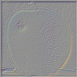
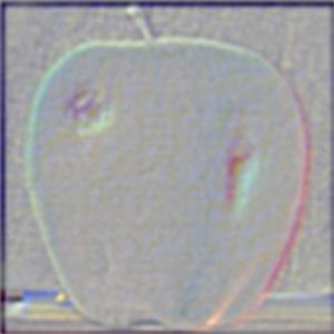
To do the blending, we create a laplacian stack for imageA and imageB, LA and LB respectively. We also create a Gaussian stack of the mask, GM. The final formula we follow to create the merge: final_img = LA*GM + (1-GM)*LB. The final image is also clipped to fall within the range of 0 and 255.