Project 2: Fun with Filters and Frequencies!
Simona Aksman
Contents
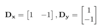
Part 1.1: Finite Difference Operator
In the first past of the project, I experimented with convolving images with their derivatives with respect to x and y in order to visualize the process of edge detection.
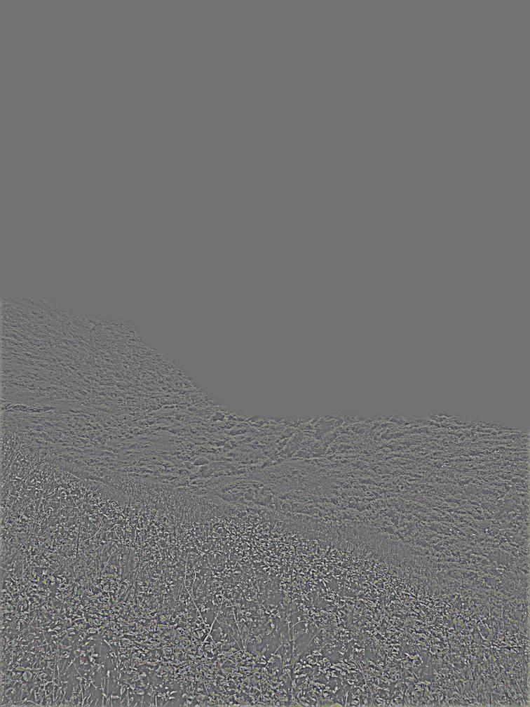
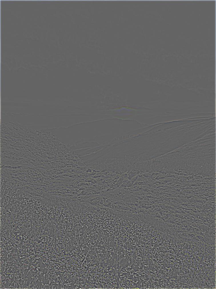
To generate an edge image, I first convolved a grayscale image with the finite difference operators, Dx and Dy, to produce partial derivatives w.r.t x and y.
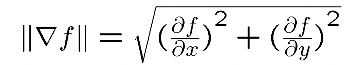
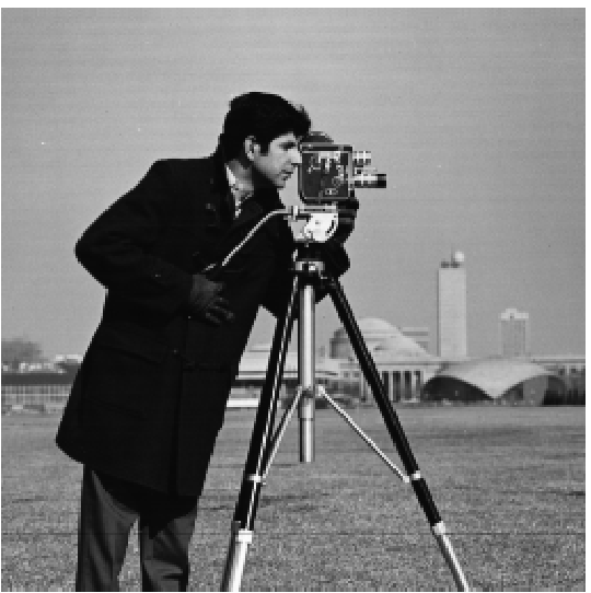
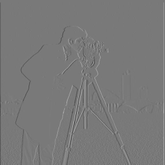
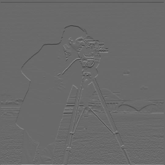
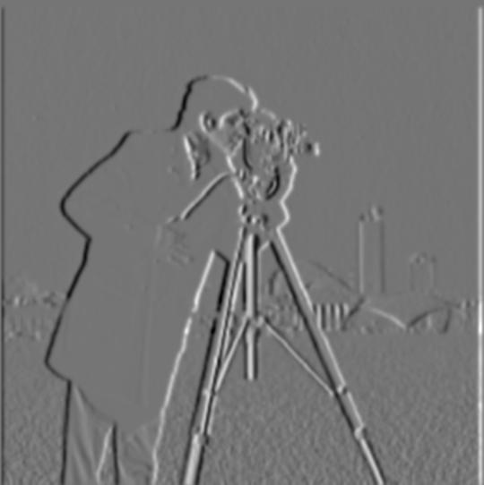
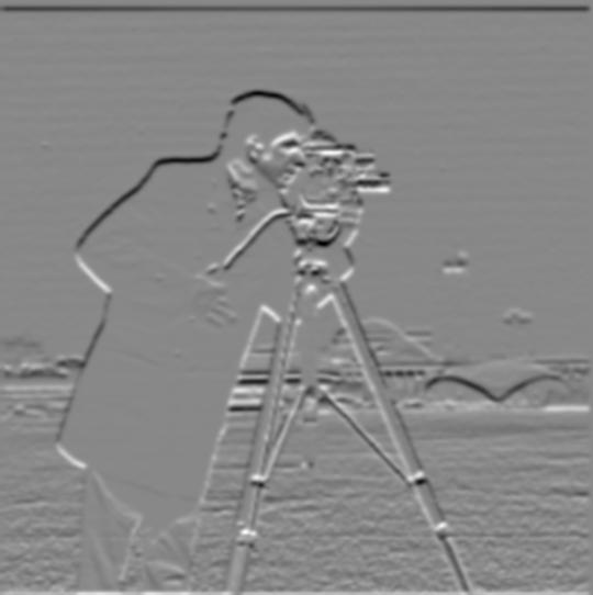
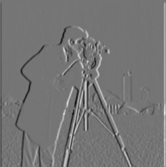
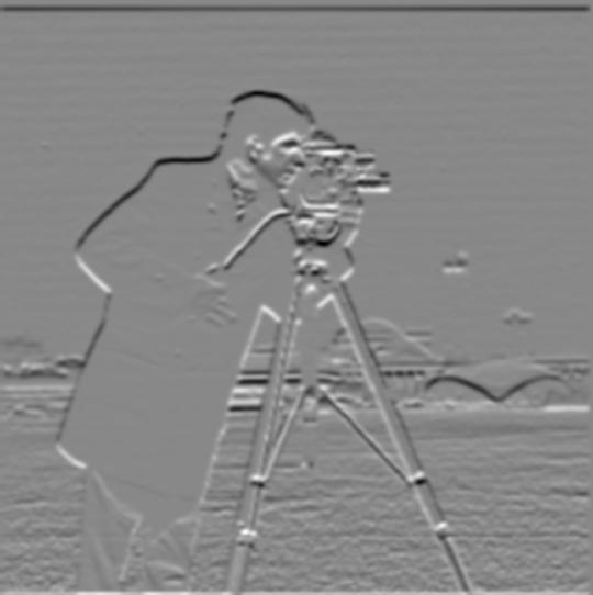
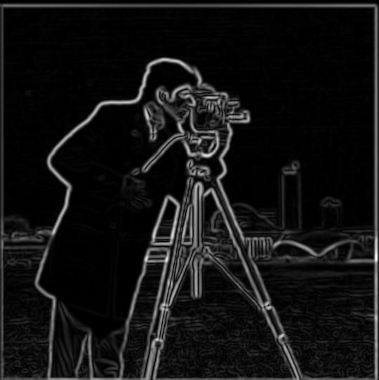
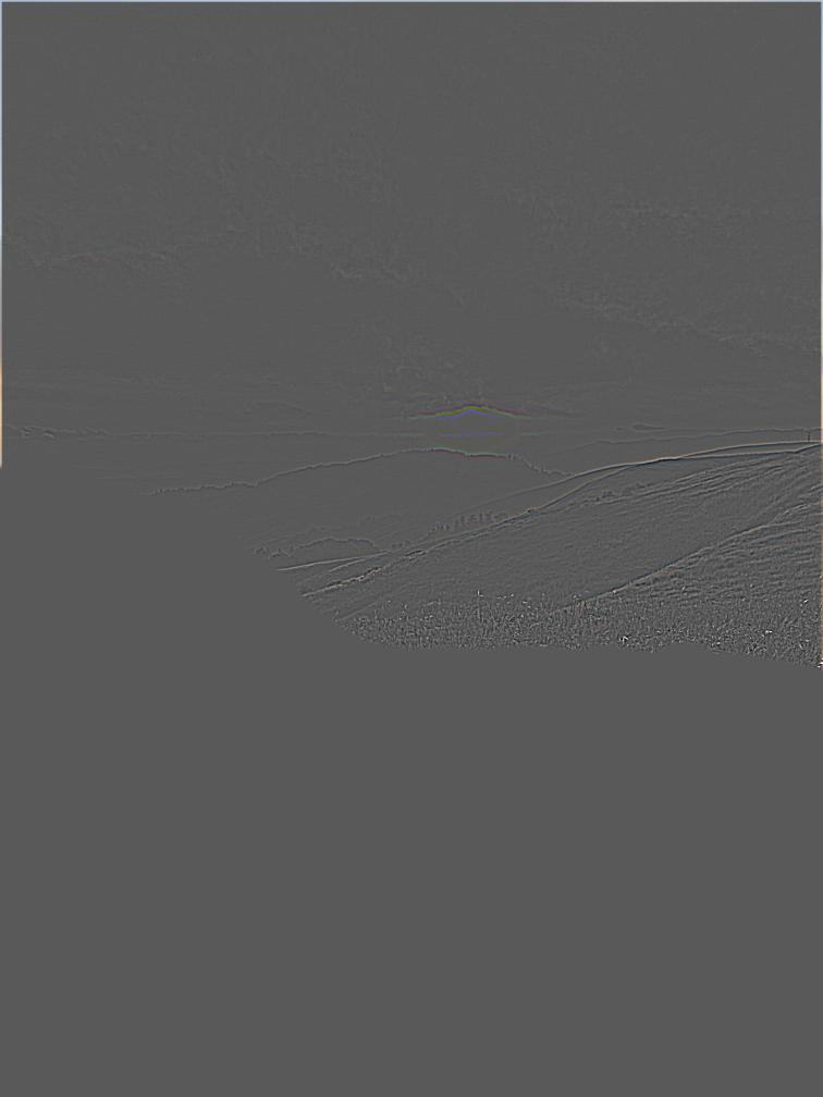
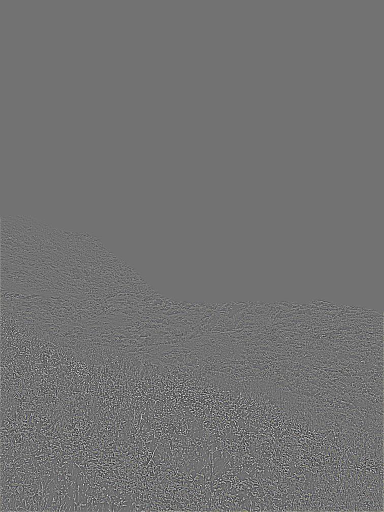
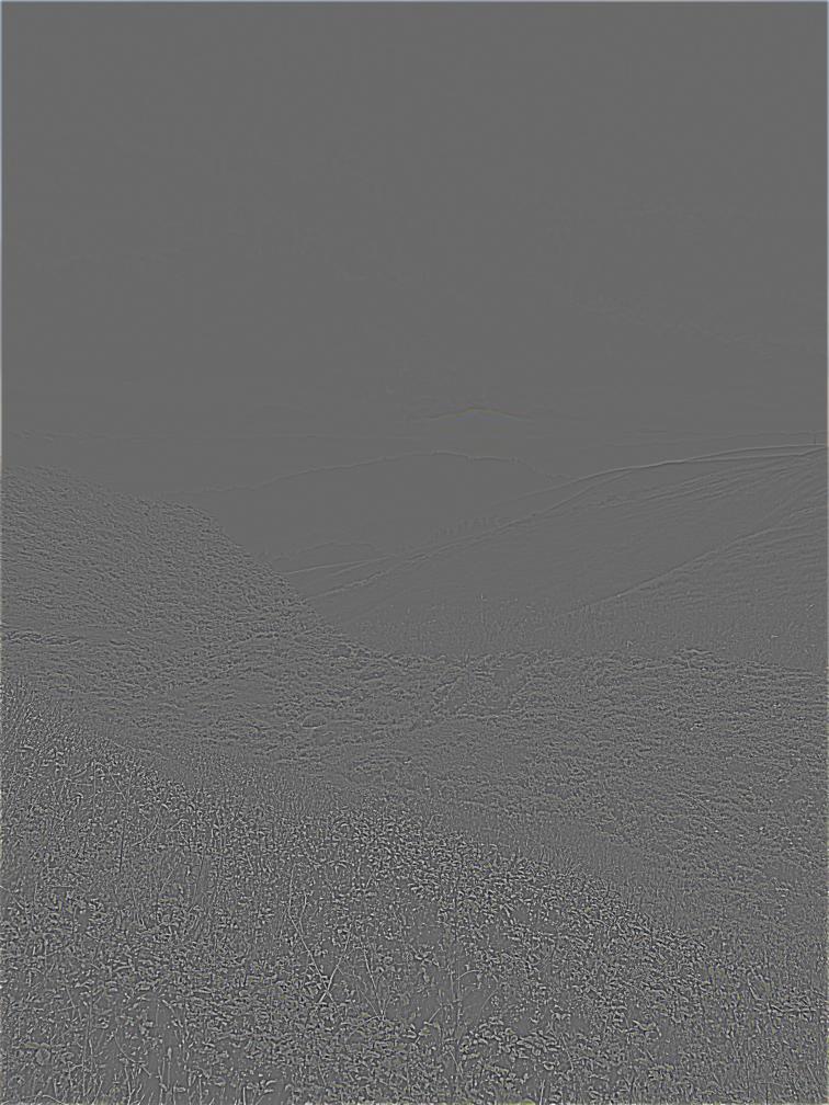
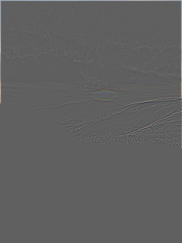
The images below visualize how the partial derivative w.r.t x pulls out the vertical edges of the image, while the partial derivative w.r.t y pulls out the horizontal edges. Using these two values, one can calculate the gradient magnitude, which is a measure of the amount of change happening in an image and therefore captures edge strength. See below for the equation for the gradient magnitude:
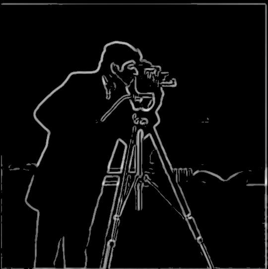
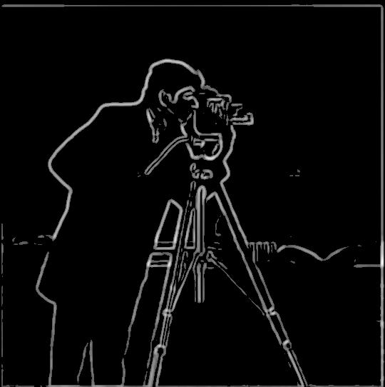
I computed the edge image by applying a threshold to the gradient magnitude in order to suppress some of the noise (non-edges) in the edge image. After trying a few values for the threshold, I decided to use 0.2. Note that even after applying this threshold, the edge image still has some noise. This issue is addressed in the next part of the project.
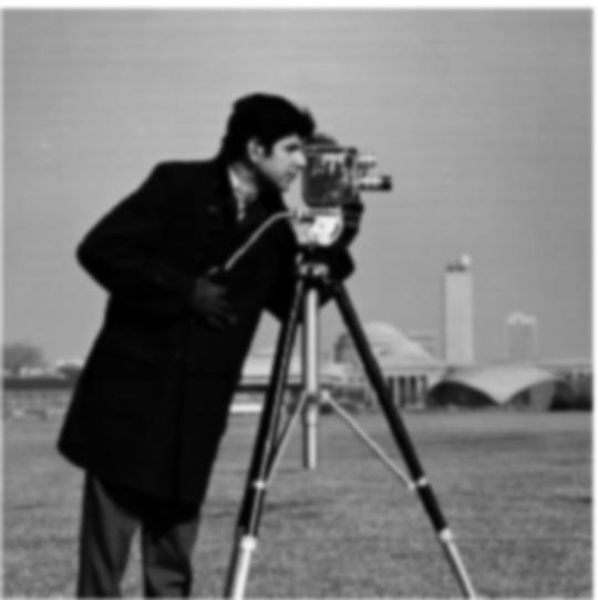
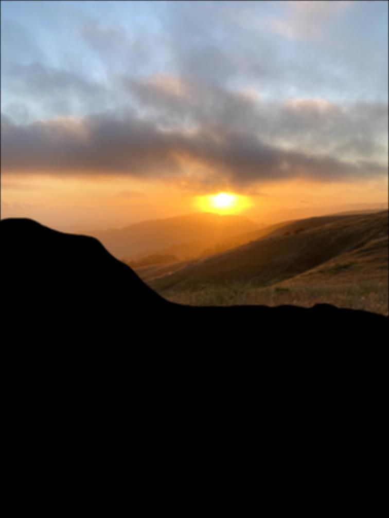
Original image
Partial derivative w.r.t x
Partial derivative w.r.t y
Gradient Magnitude
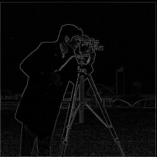
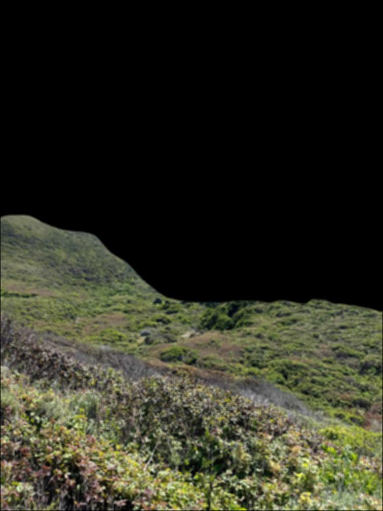
Edge image
Part 1.2: Derivative of Gaussian (DoG) Filter
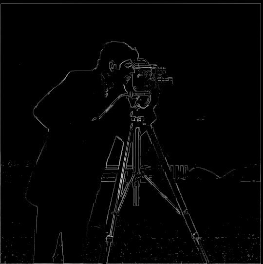
I was able to fix the noise issue I encountered in part 1.1 by applying a Gaussian filter first. I tried two different approaches to applying this filter. Using method 1, as shown below, I first blurred the grayscale image with a Gaussian filter and then applied the derivative w.r.t x and y directly. Then I computed the gradient magnitude and binarized the edges with a threshold. In this case, the threshold I picked after some experimentation was 0.05. In addition to having fewer noisy artifacts on the image, the edge image produced using method 1 also has more well-defined edges than the edge image produced in part 1.1. I also noticed that the range of pixel values in the edge image is much smaller than in the edge image produced in part 1.1, perhaps because some high frequencies have been removed by the Gaussian blur.
Next I tried to achieve the same result using method 2, by which I convolved the Gaussian filter directly with the derivatives w.r.t x and y, and then computed the gradient and edge images from the product of the image and the convolved Gaussian derivatives. I used the same threshold value of 0.05 for method 2 and was able to produce a similar-looking result. See below for the step by step process for applying each method.
Method 1:
1. Apply a Gaussian blur to original image
2. Convolve Gaussian image with derivative w.r.t x
3. Convolve Gaussian image with derivative w.r.t y
4. Compute gradient magnitude

5. Binarize edges to produce edge image
Method 2:
1. Convolve Gaussian kernel with derivative w.r.t x

2. Convolve Gaussian kernel with derivative w.r.t y

3. Convolve image with the output of step 1
4. Convolve image with the output of step 2
5. Gradient Magnitude
6. Edge image
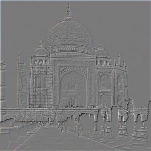
Part 2.1: Image "Sharpening"
In this part of the project I learned how to create an unsharp mask filter in order to "sharpen" edges in images. You can do this by subtracting a Gaussian filtered (low frequency) version of an image from the original image, and then adding it back to the original image. This process adds extra high frequencies to an image and can be expressed via the following equation:
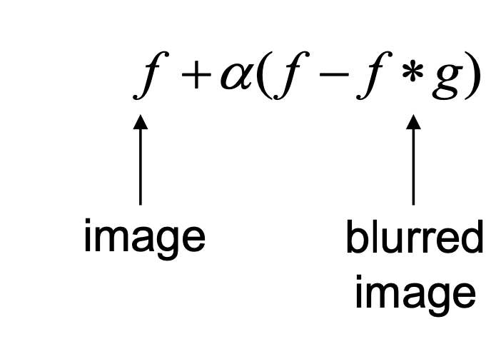
where α (alpha) is the parameter that determines the magnitude of high frequencies that are added back. I experimented with various images and alpha parameters and included some of the results of these experiments below.
Note that in all the examples below, I have included the sigma and kernel parameters I used to generate the image. These parameters control the height and width of the Gaussian blur.
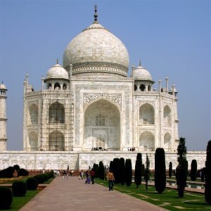
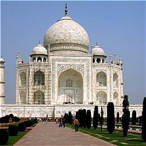
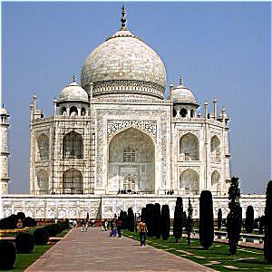
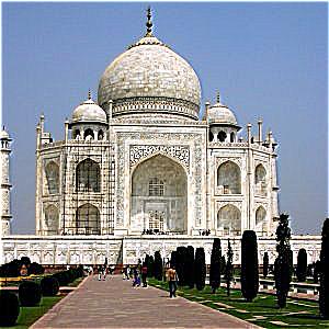
taj.jpeg
sigma = 1kernel = 6
Original image
Low Frequency

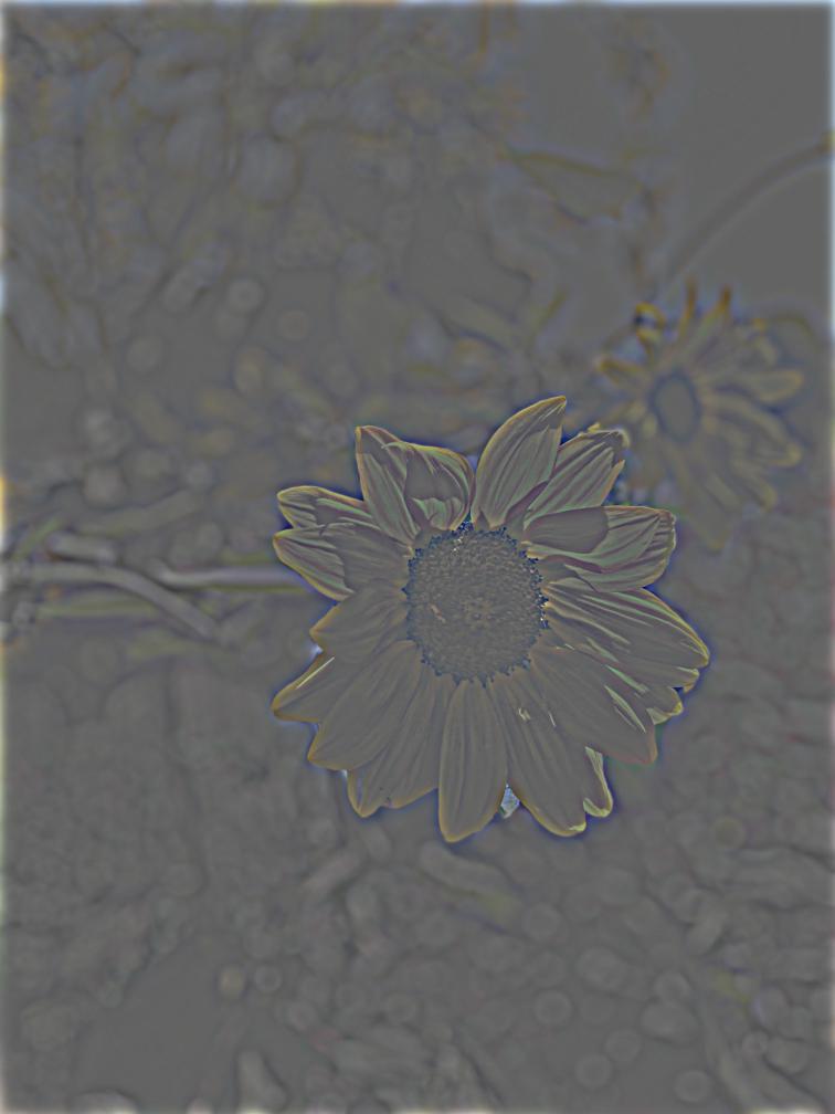
High Frequency
Sharpened, α = 1
Sharpened, α = 2
Sharpened, α = 3
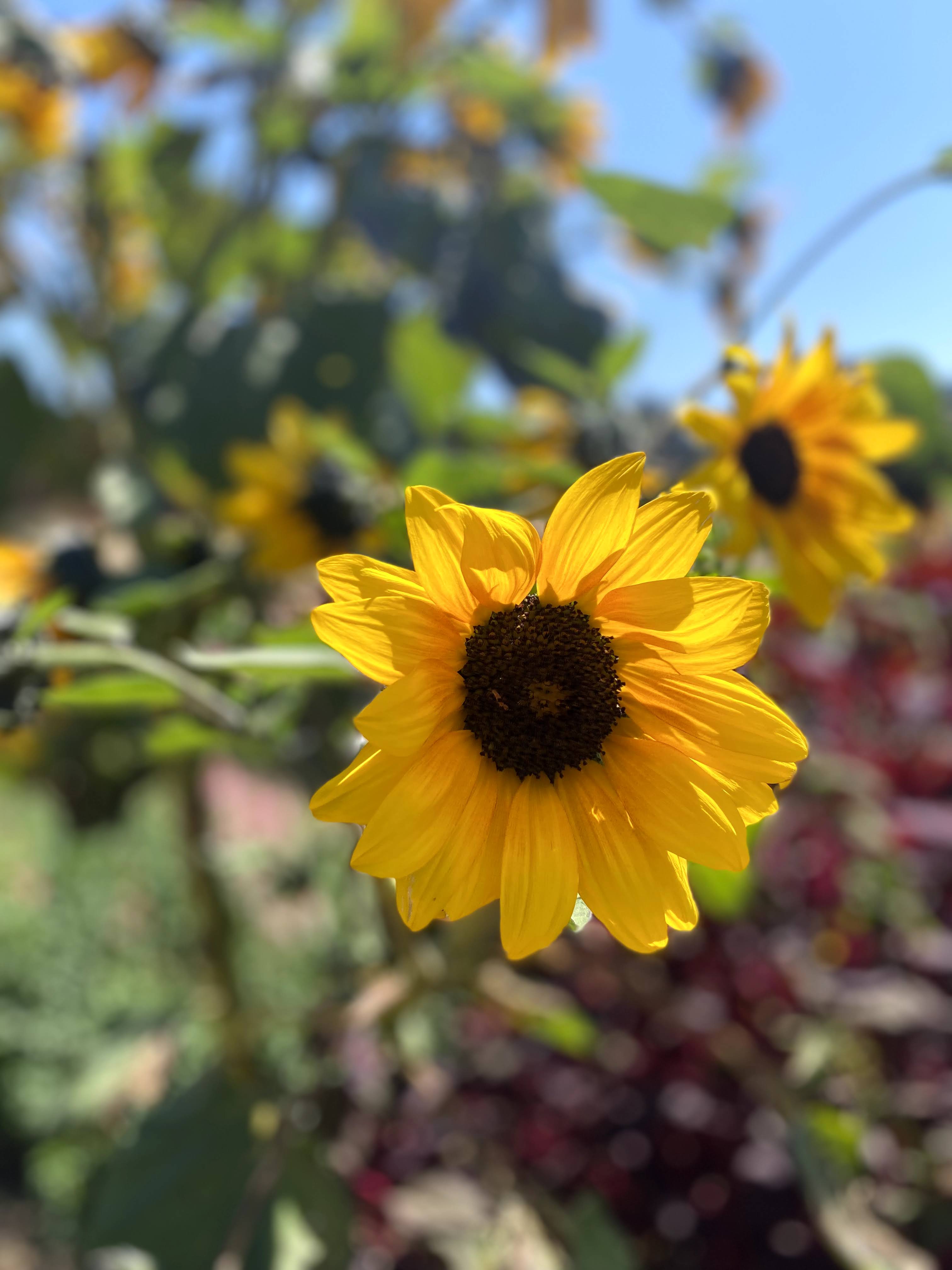
flower.jpeg
sigma = 5kernel = 30
Original image
Low Frequency
High Frequency
Sharpened, α = 1

Sharpened, α = 2

Sharpened, α = 3
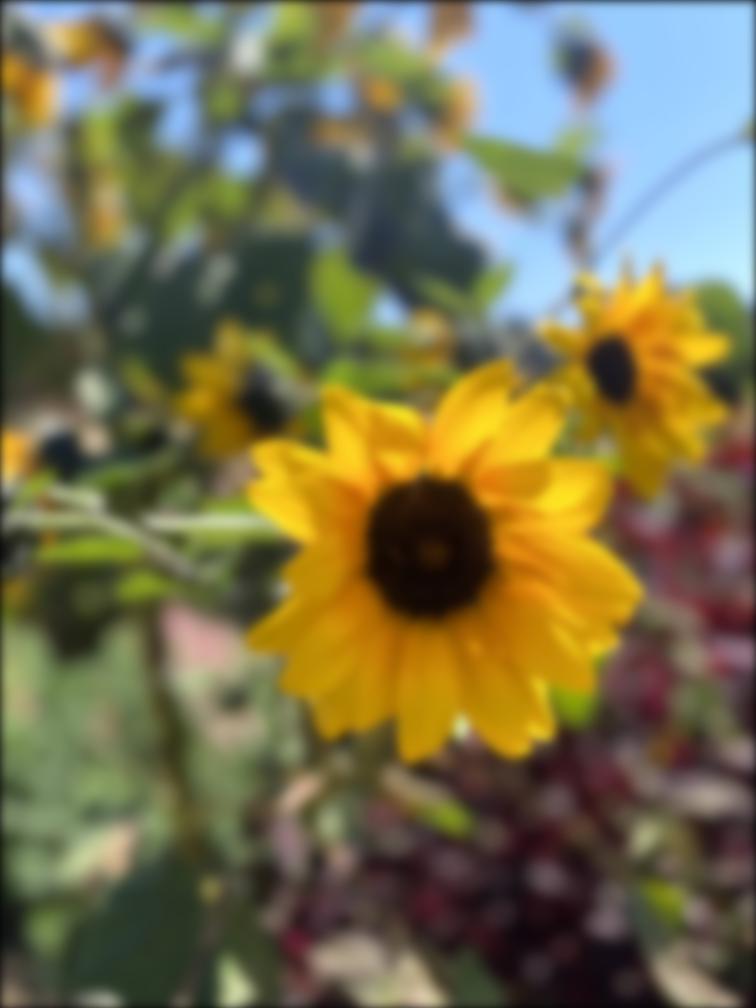
I attempted to blur and then sharpen an image to see whether I could recover the original image. See below for an example of this process. It appears that the "resharpening" process did not recover the original image. The new image is blurrier than the original, and its border has been altered due to the transformations.
Original image
2. After Gaussian blur
sigma = 2
kernel = 12
3. Resharpened
sigma = 2
kernel = 12
alpha = 4
Part 2.2: Hybrid Images
Next, I generated hybrid images, which utilize a human perceptual phenomenon called contrast sensitivity to display different images depending on the viewer's distance from the image. You can produce this hybrid image effect by blending the high and low frequency bands of two different images. See below for some of the hybrid images I generated.
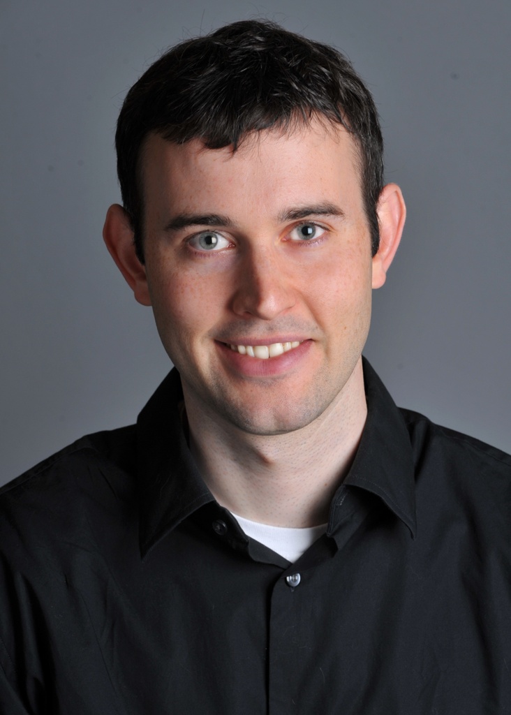
Derek
Nutmeg
Hybrid of Derek and Nutmeg
sigma1 (Derek) = 20
sigma2 (Nutmeg) = 25
kernel = 20
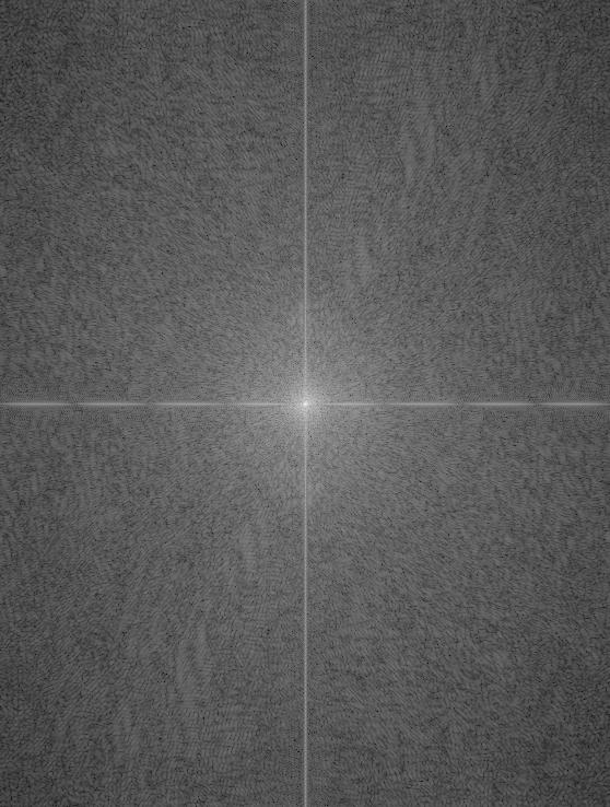
Fourier analysis
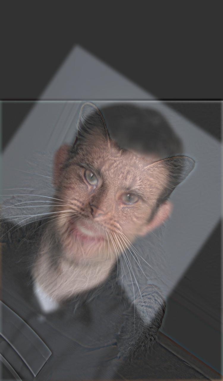
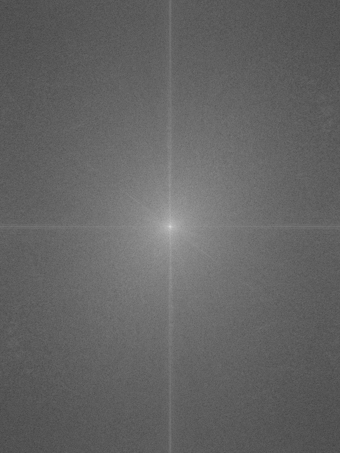
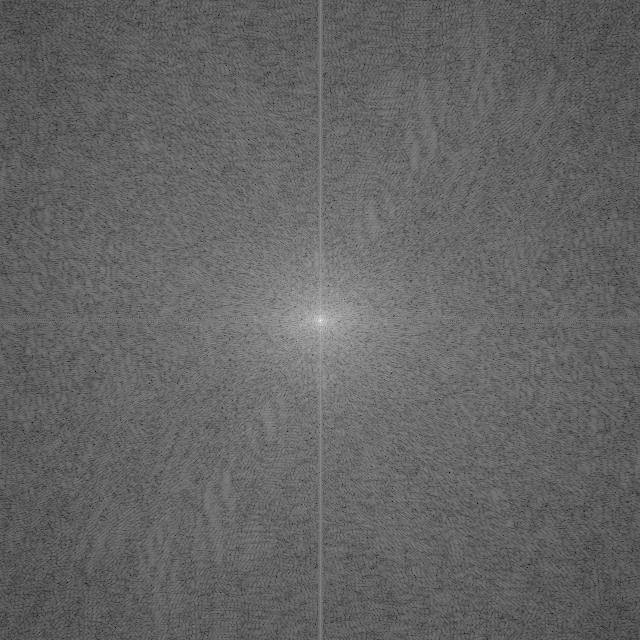
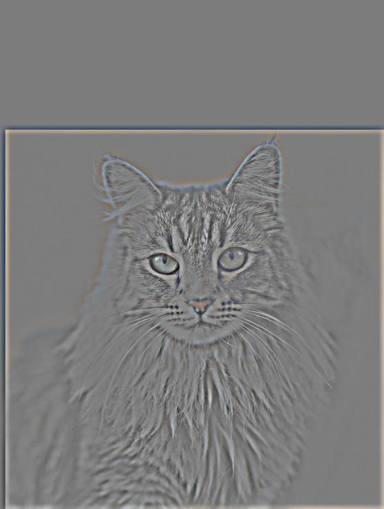
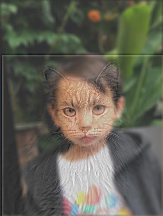
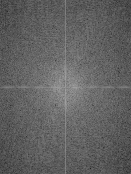
One of my favorite parts of project 2 was generating hybrid images of my niece of and nephew (with their permission). See below for some of my results. In the first example, I turn my grumpy nephew Jojo into a cat. I also applied a Fourier transform to grayscale versions of the images to help visualize the different frequency ranges of each part of the process. You can see that the original images, the lowpass (low frequency band) image, and the final image have a strong concentration of low frequencies, whereas many of the low frequencies have been removed from the highpass (high frequency band) image of the cat.
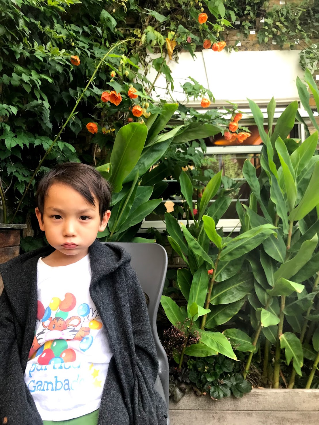
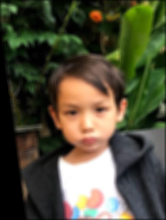
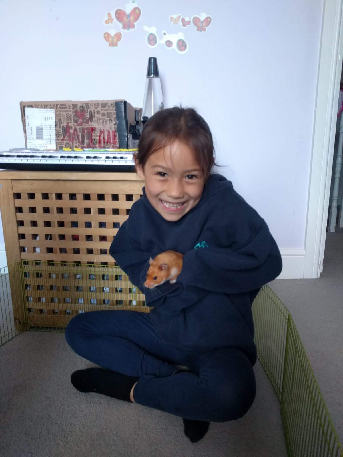
My nephew Jojo
Lowpass of Jojo
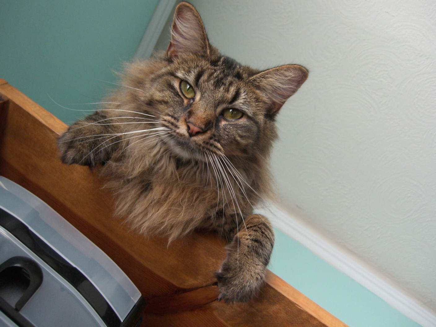
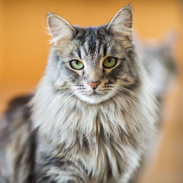
A cat
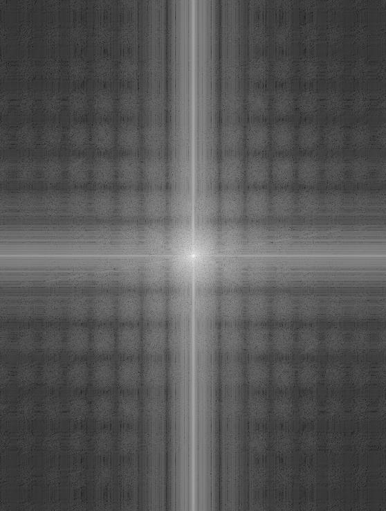
Highpass of the cat
Hybrid of Jojo and the cat
sigma1 (Jojo) = 20
sigma2 (Cat) = 15
kernel = 15
Unfortunately, the hybrid of my niece Clara and a baby corgi was less successful because the images were not too compatible (the corgi's body is very short compared to Clara's).
My niece Clara
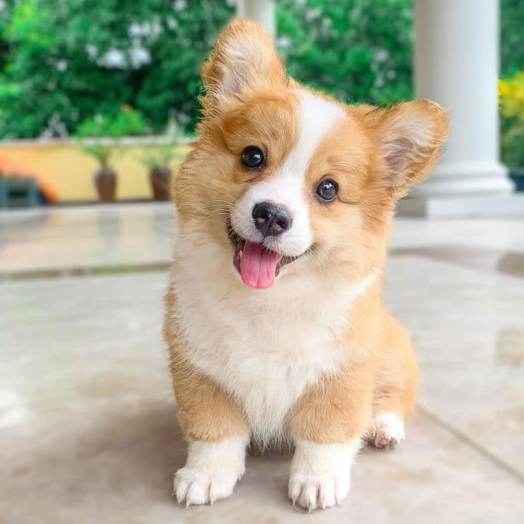
A baby corgi
Hybrid of Clara and a corgi
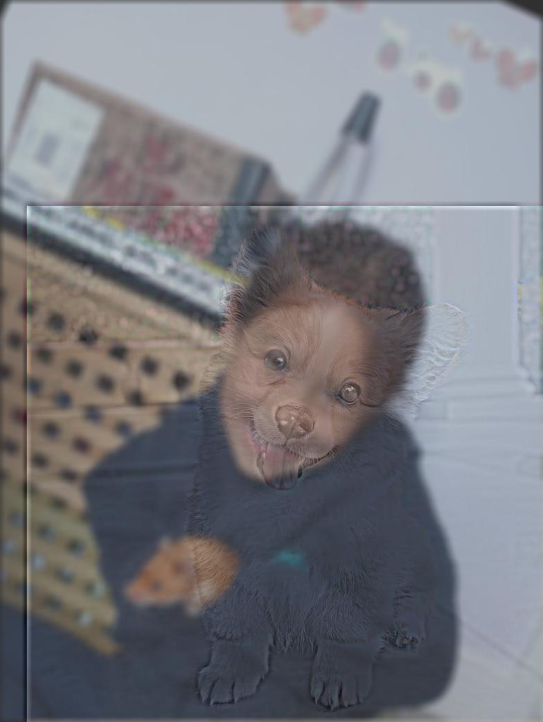
sigma1 (Clara) = 20
sigma2 (Corgi) = 15
kernel = 15
Testing color
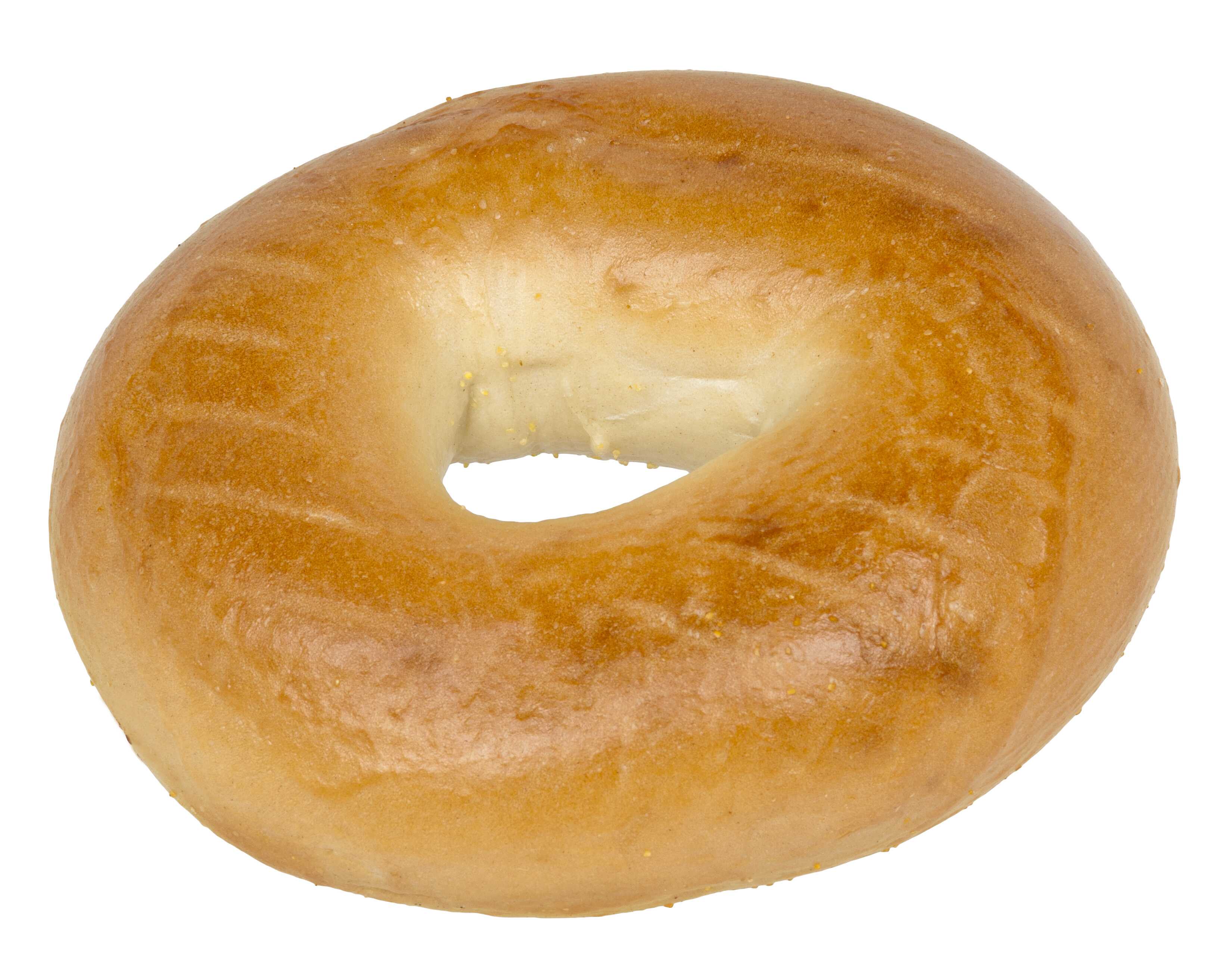
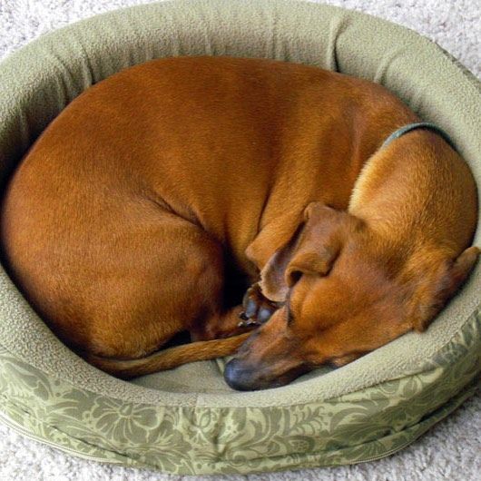
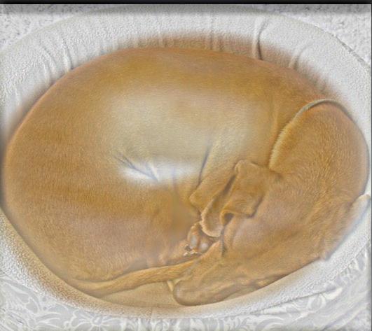
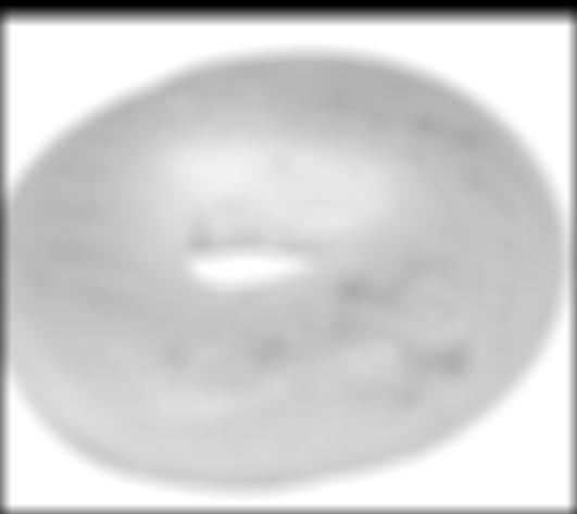
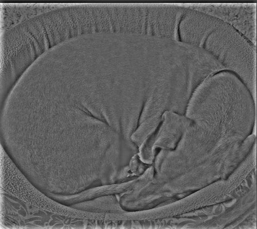
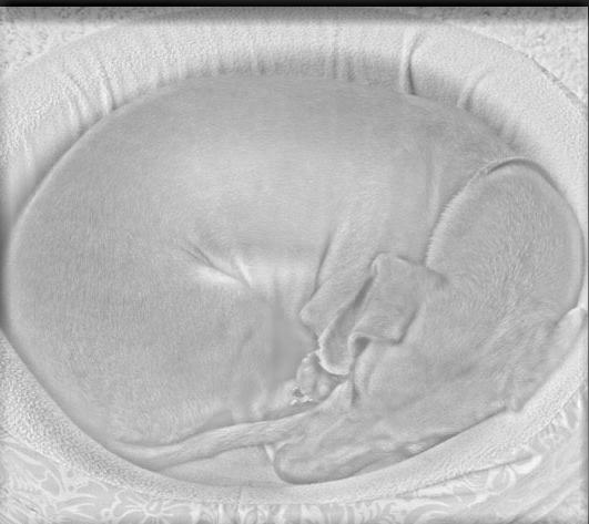
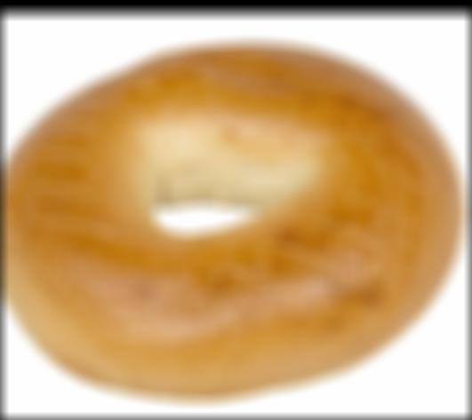
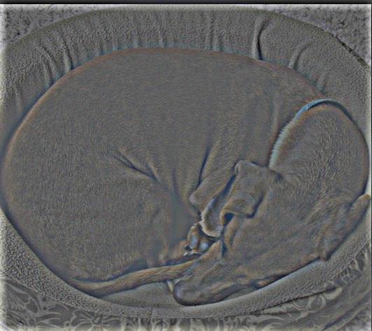
I created hybrid images in both grayscale and color and found that the high frequency component generally did not retain a lot of color, and so the hybrid image mostly took on the colors of the lowpass image. You can see this in the example of the hybrid bagel dog below. The colors of the dog's bed, for instance, are completely missing in the final image.A bagel
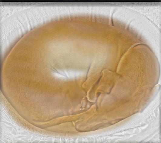
A curled up dog
Hybrid of a bagel and a dog
sigma1 (Bagel) = 15
sigma2 (Dog) = 25
kernel = 20
Grayscale
Color
Part 2.3: Gaussian and Laplacian Stacks
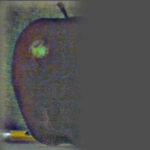
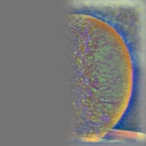
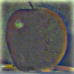
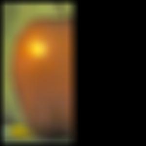
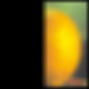
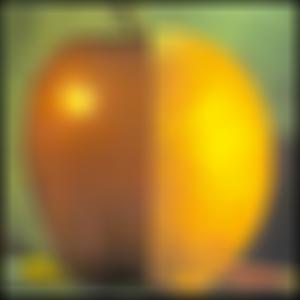
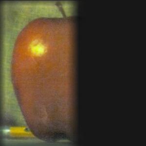
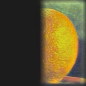
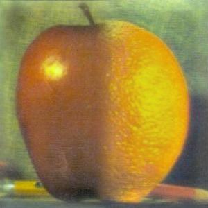
In this part of the project, I learned how to implement Gaussian and Laplacian stacks, which can be used to blend two similar images smoothly. A stack is a series of filters applied iteratively to an image. A Laplacian stack is computed by applying a Gaussian blur at each layer of the stack and then subtracting that Gaussian image from the input image at that layer. The image retains it's original dimensions at each level of the stack. One important property of a Laplacian stack is that the last level must be equivalent to the Gaussian stack at that level in order to recover the original image. In the figures below, I have recreated the blending process for the oraple using Gaussian and Laplacian stacks.Layer 0
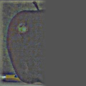
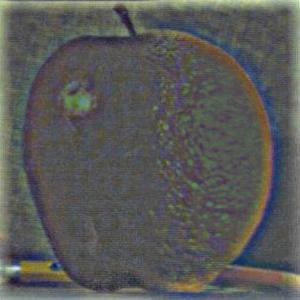
Apple
Orange
Oraple
Layer 2
Layer 4
Outcome
Part 2.4: Multiresolution Blending
Next I replicated the multiresolution blending algorithm outlined by Burt and Adelson in their 1983 paper using the stacks I developed for part 2.3. Given two images A and B and a mask M, you can produce a splined image LS where each level L of a stack using the following equation:LSL = GRL * LAL + (1 - GRL) * LBL
where LS is the spline for each level L, GR is the Gaussian mask at L, and LA and LB are the Laplacian versions of images A and B at L.
See below for some examples that worked. I found it challenging to create a blended image that looked natural, because it relies on the images being similar enough for the spline to make sense. For both examples below I used the parameters sigma = 5 and L = 5.
Layer 0
Layer 2
Layer 4
Outcome
Reflections
This project taught me how to transform images in creative and interesting ways using filters and frequencies. In addition to this project being fun, it also helped me gain a stronger conceptual understanding of key image processing concepts, such as Fourier transforms.
Some images were found online. Sources:
[1] https://www.boredpanda.com/cooper-and-baby-corgi/
[2] https://www.goodhousekeeping.com/life/pets/g26898596/
large-cat-breeds/
[3] https://en.wikipedia.org/wiki/New_York_style_bagel
[4] https://www.pinterest.com/pin/386746686735429865/