Jeremy Warner — jeremy.warner at berkeley.edu

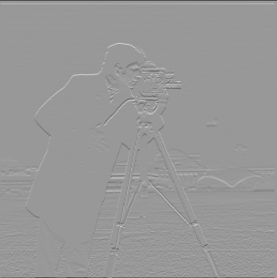
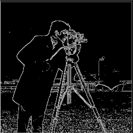
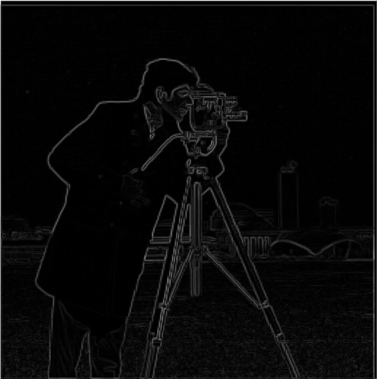
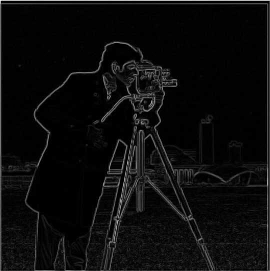
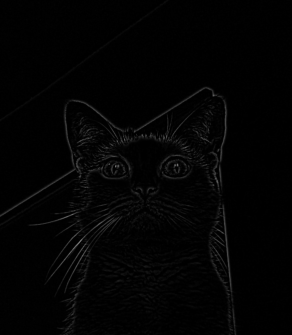
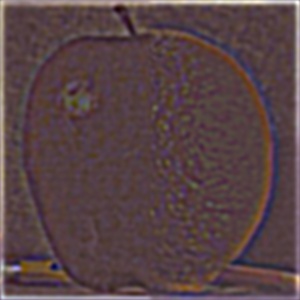
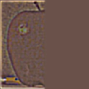
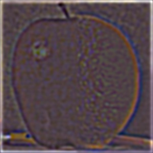
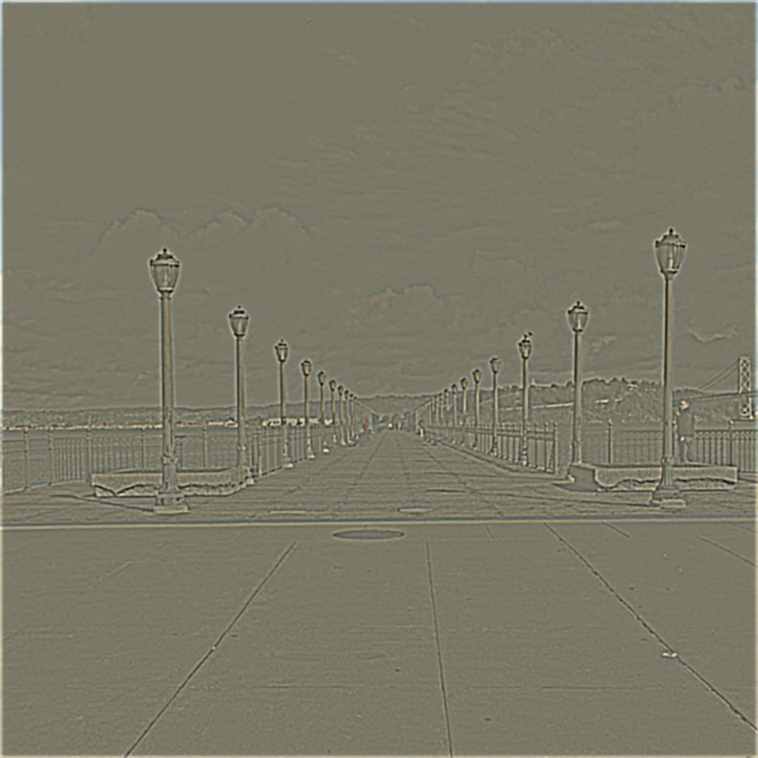
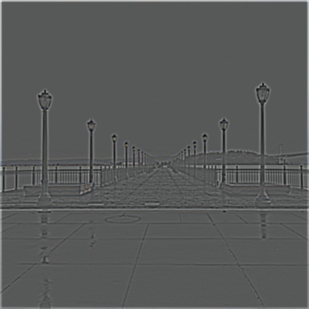
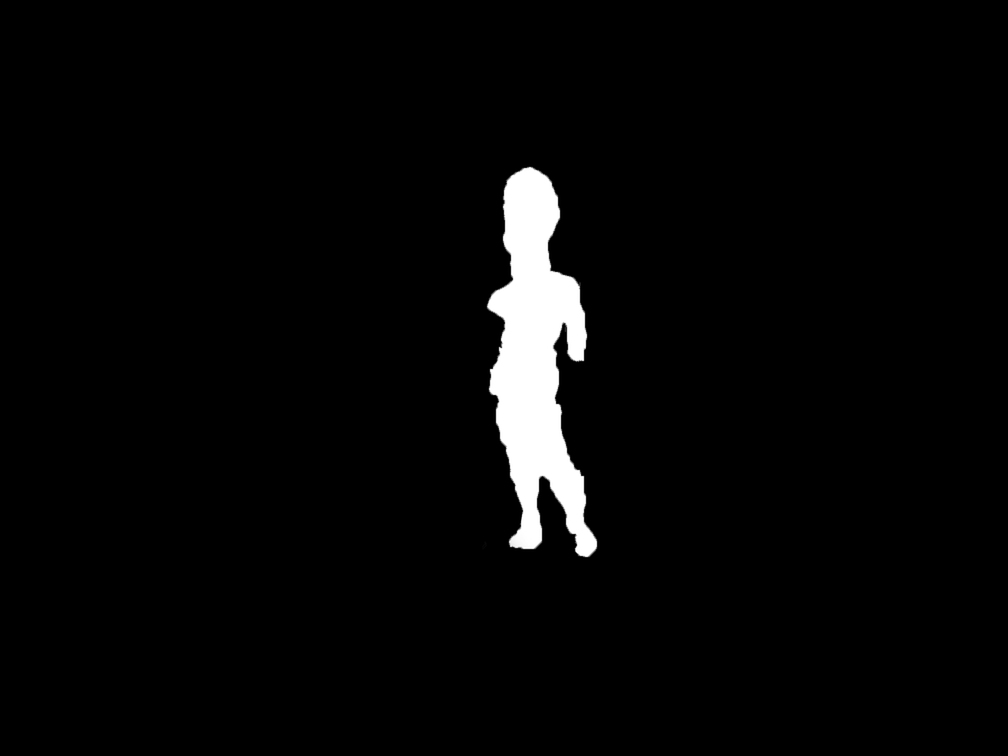
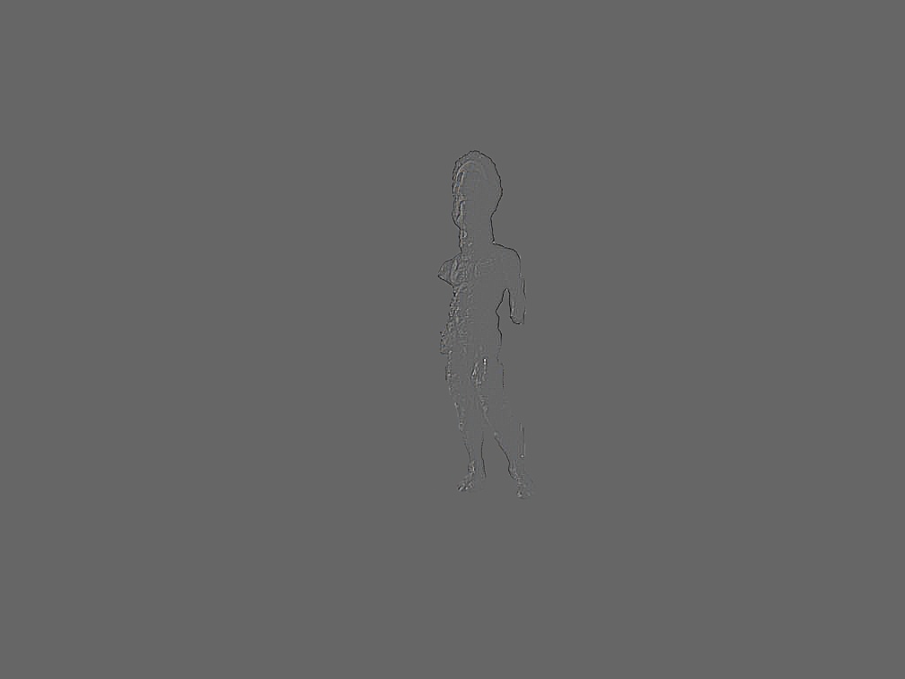
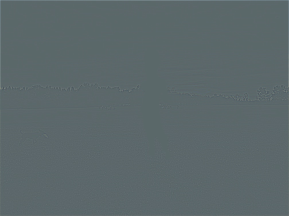
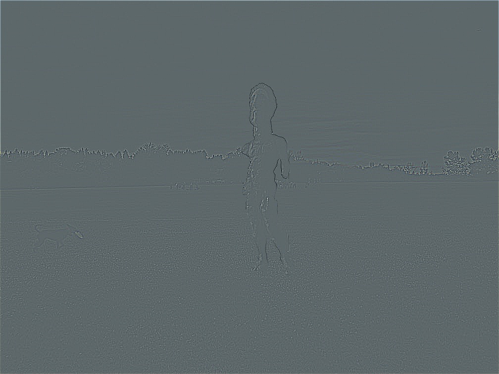
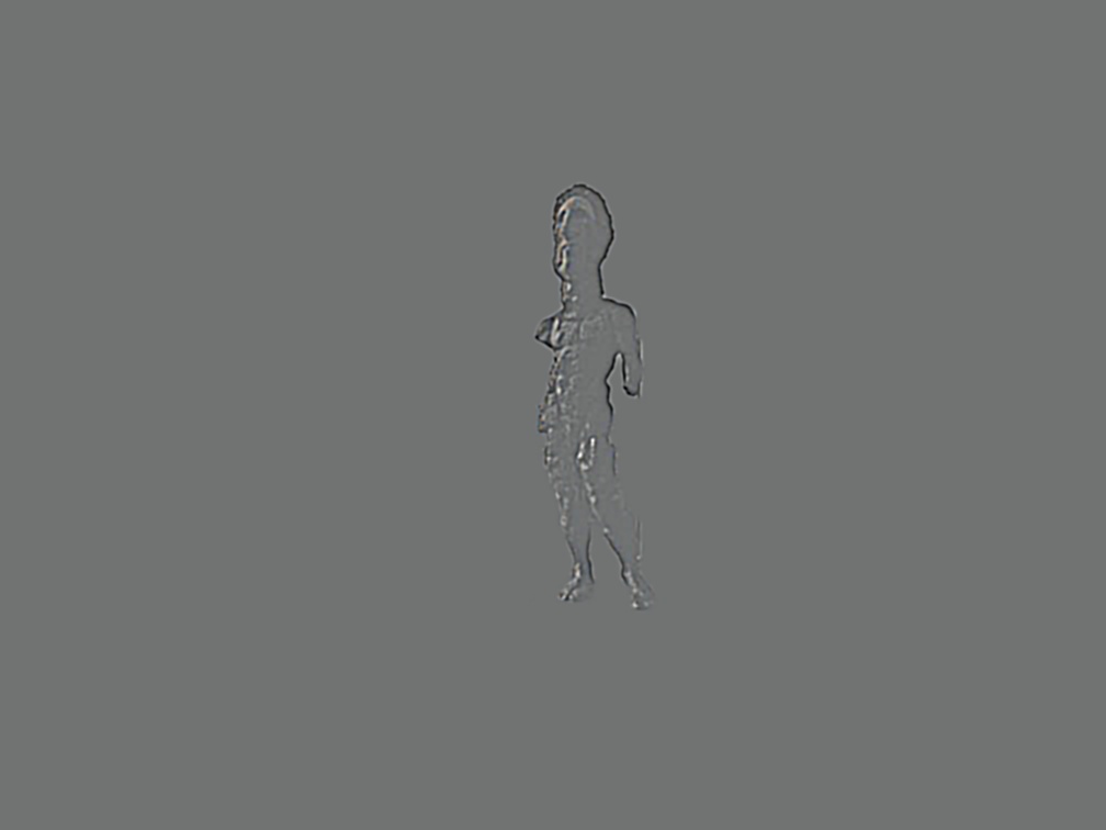
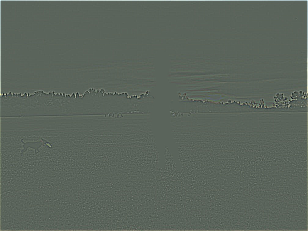
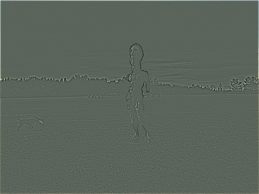
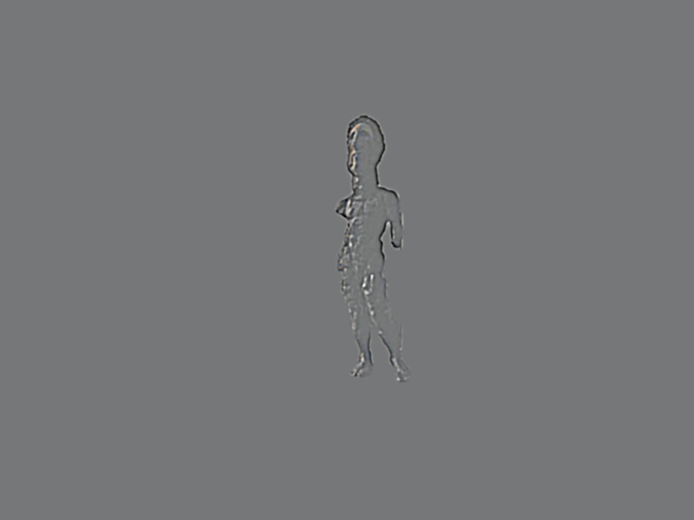
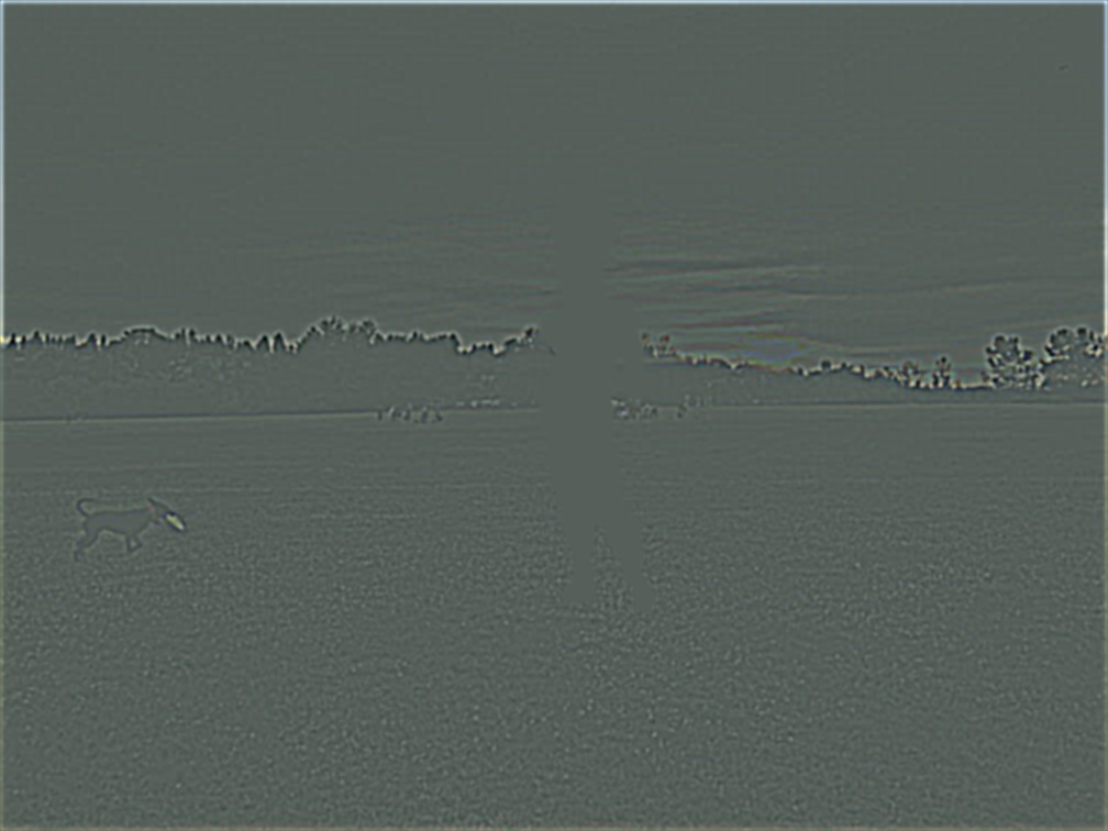
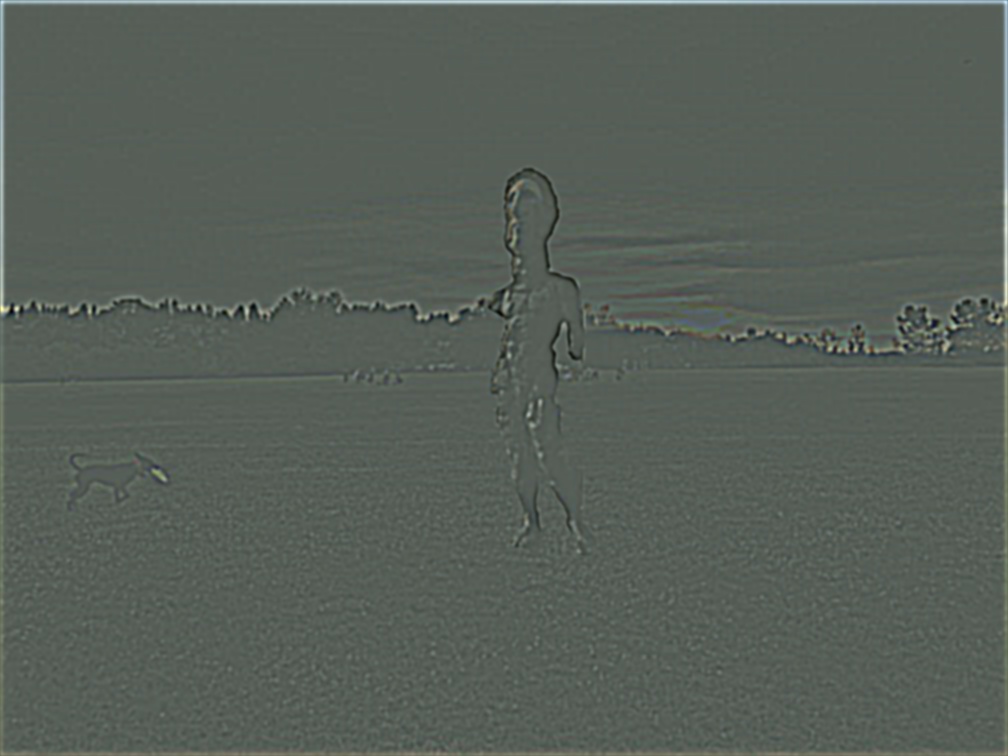
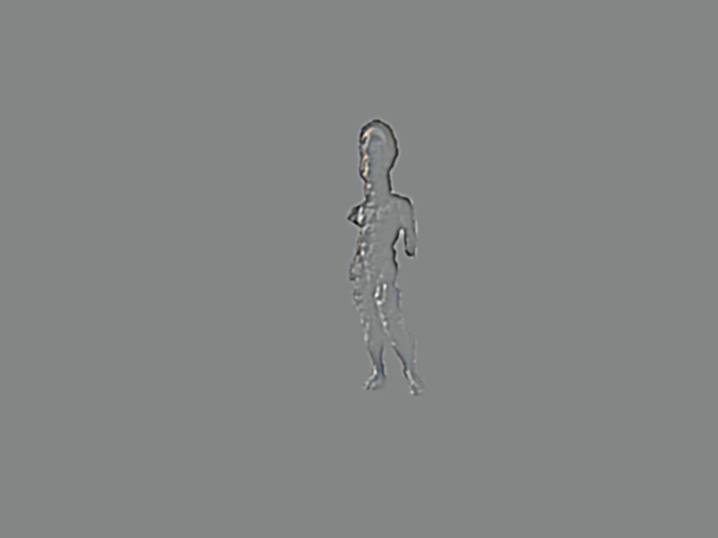
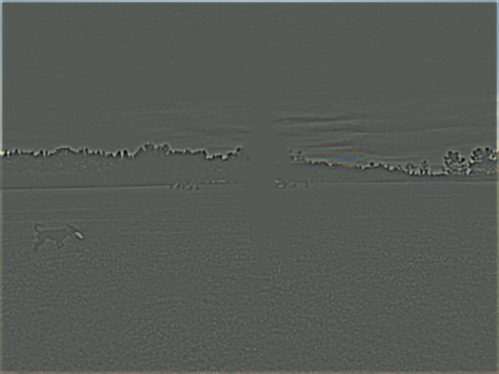
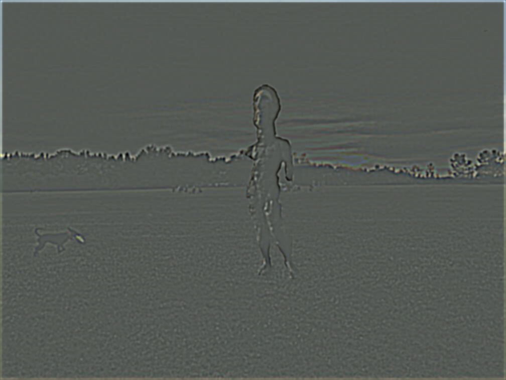
I found that a threshold of 25 worked well enough to filter out a good amount of the noise from the grass in the foreground while also sketching out the building edges in the background. Depending on you wanted to focus on, you could choose a higher or lower threshold. For example, if you wanted to capture the soft grey edge of the building in the background you could lower the threshold but then the noise from grass would increase.
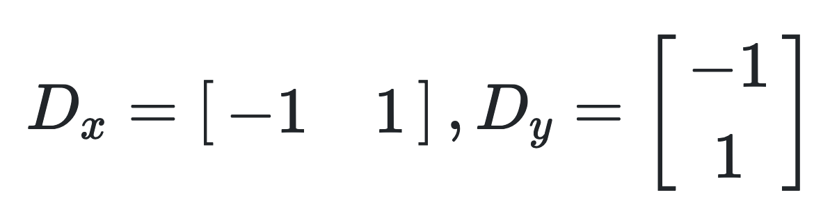
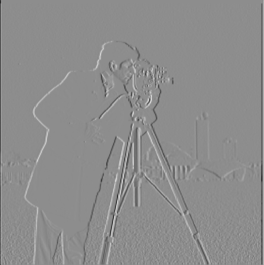
Gradient Magnitude Computation: grad = np.sqrt(dx**2 + dy**2). Computing this gradient is straightforward, though note that there is not information on direction, which means edge orientation is lost by only considering the magnitude of the gradient.
I use the Gaussian kernel to blur these images (3x3). Unless specified, I have cv2.getGaussianKernel set the value of sigma based on their built-in equation, which bases it off of the kernel size: sigma = 0.3*((ksize-1)*0.5 - 1) + 0.8

What differences do you see?
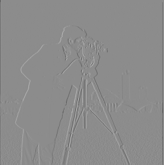
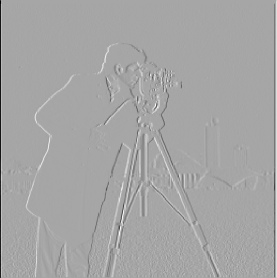
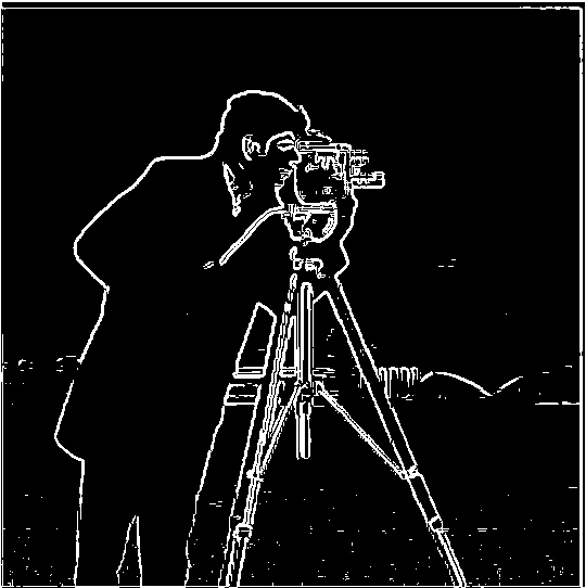
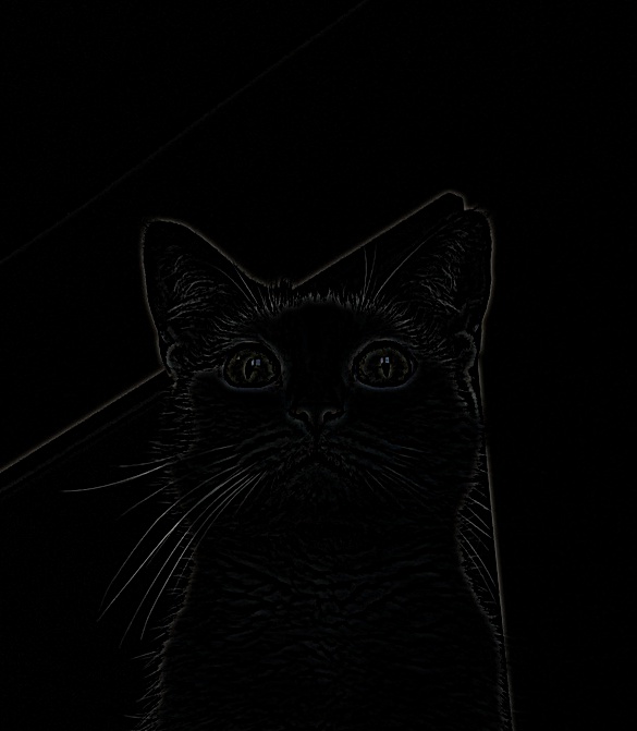
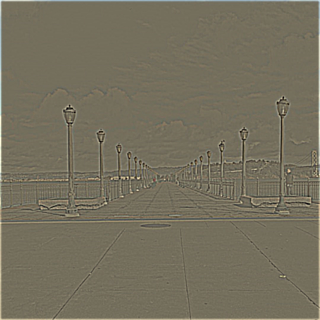
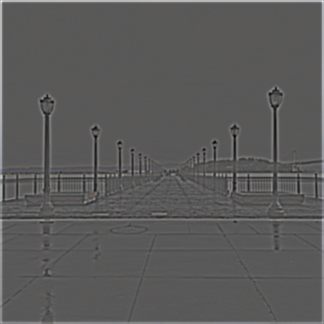
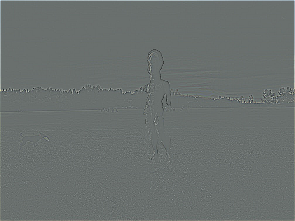
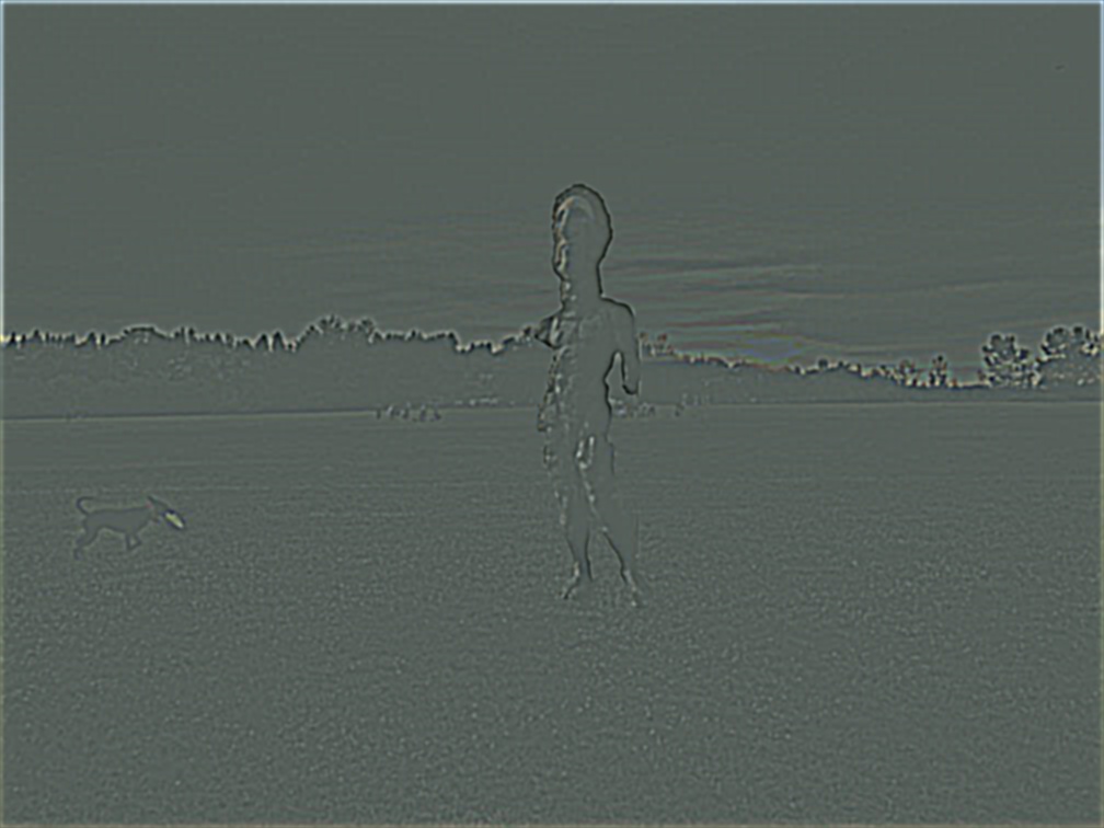
Using the same threshold, there is much less noise (no grass lines are visible). Additionally, the original edges seemed to have many jagged edges where they go back and forth near the camera tripod legs, but this effect is removed with blurring the source image. After applying the blur, edges in the image are much smoother. This is especially noticable around the cameraman’s face and eyes. Repeating the process from part 1.1:
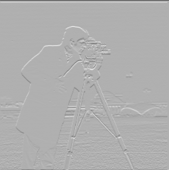
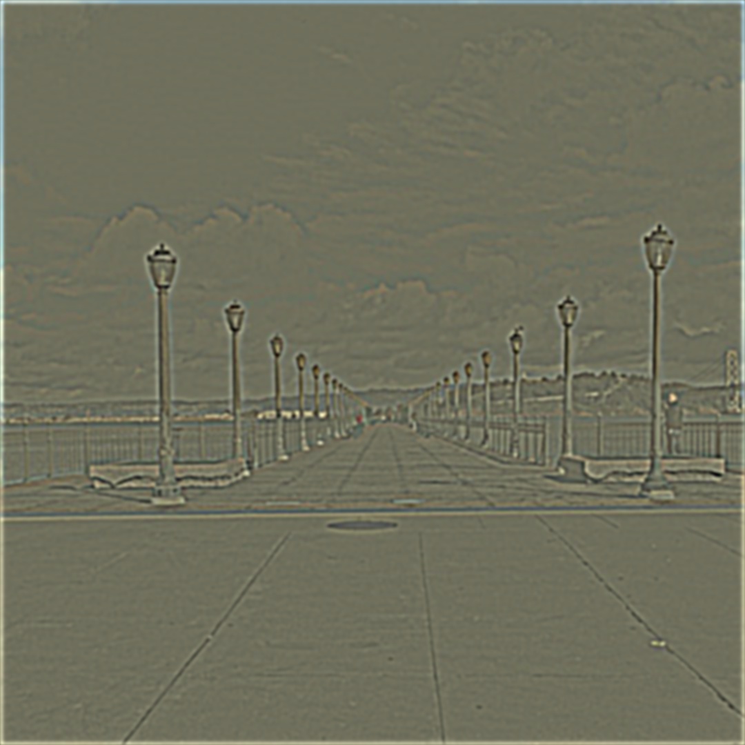
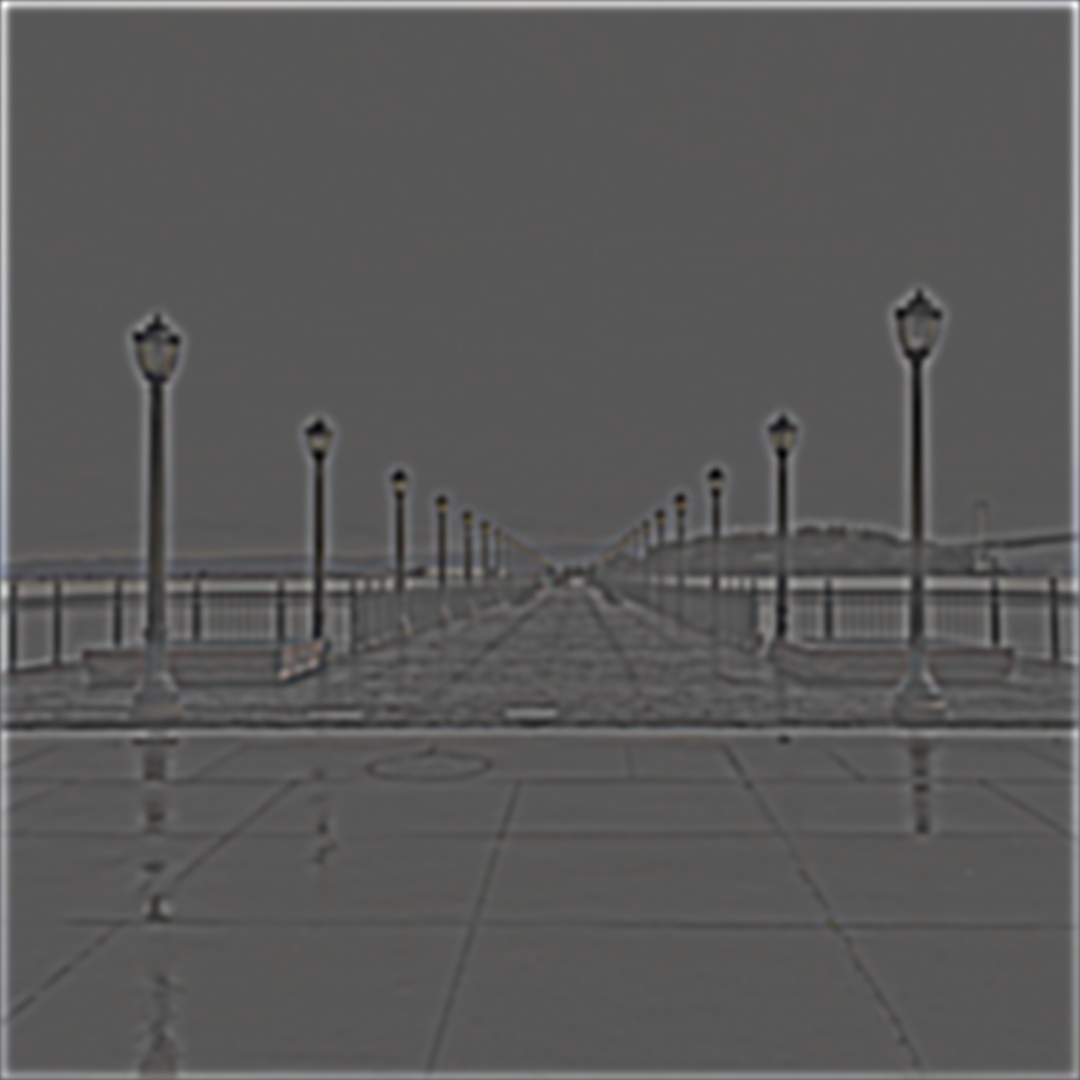
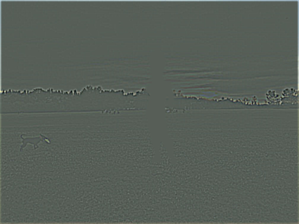
Using the DoG filter, we can do the same process with a single convolution.


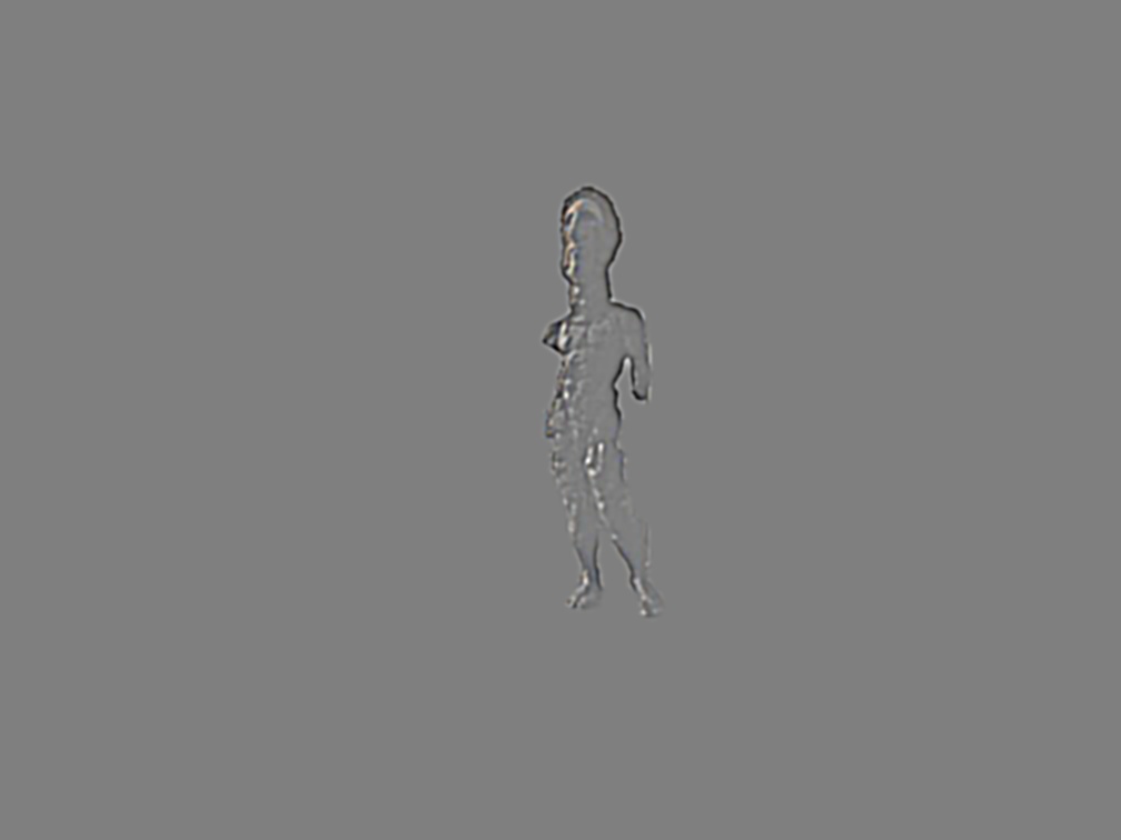
Verify that you get the same result as before.
We can see that applying the DoG has the same effect:

We create an unsharp filter according to the project specification. The equation for doing this with a single convolution filter and the Laplacian of Gaussian is:
LoG = (1+α) * e − α * gk
where:
For this section, I used a Gaussian kernel of size 5x5 unless otherwise noted.
taj.jpgOriginal 
α = 1 
α = 3 
α = 9 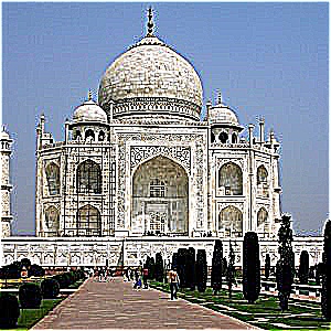
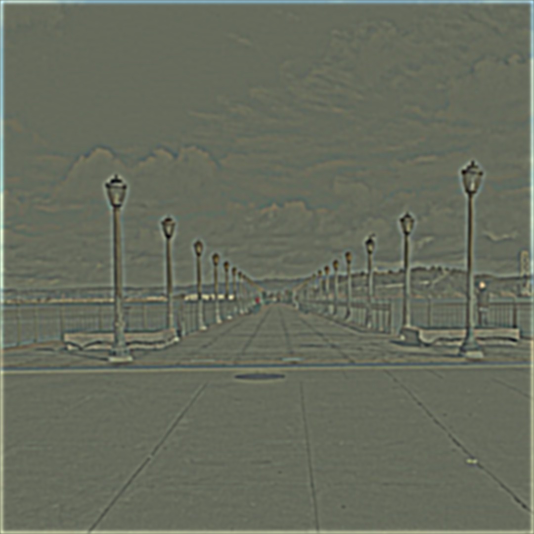
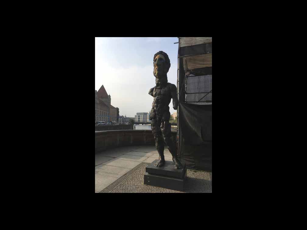
Applying this filter to a picture I took from the Berkeley fire trails:
Original 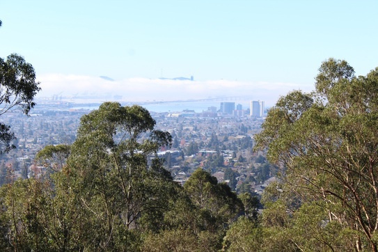
α = 1 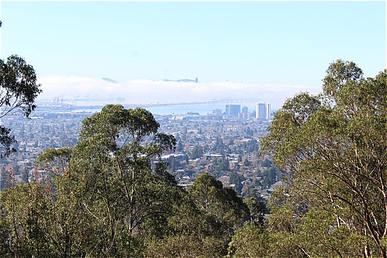
α = 3 
α = 9 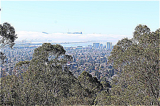
The image here is of Zabriskie Point in Death Valley National Park (source). For this section, I use a 9x9 Gaussian kernel. This makes the effect of the blurring and sharpening even more pronounced. Adding in a higher level of alpha after blurring lets us recover some of the original detail that is hidden when using the Gaussian blur. This is noticeable in the patches of dirt that are removed in the blurred image but reappear in the sharpened image, which almost emulates the effect of adjusting a camera’s focal length. However, there is still a clear difference in the blurred and resharpened images due to reduced high frequency information.
Original 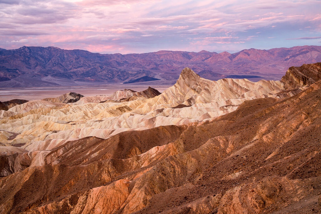
Blurred 
α = 1 
α = 3 
α = 9 
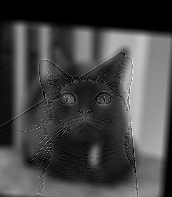
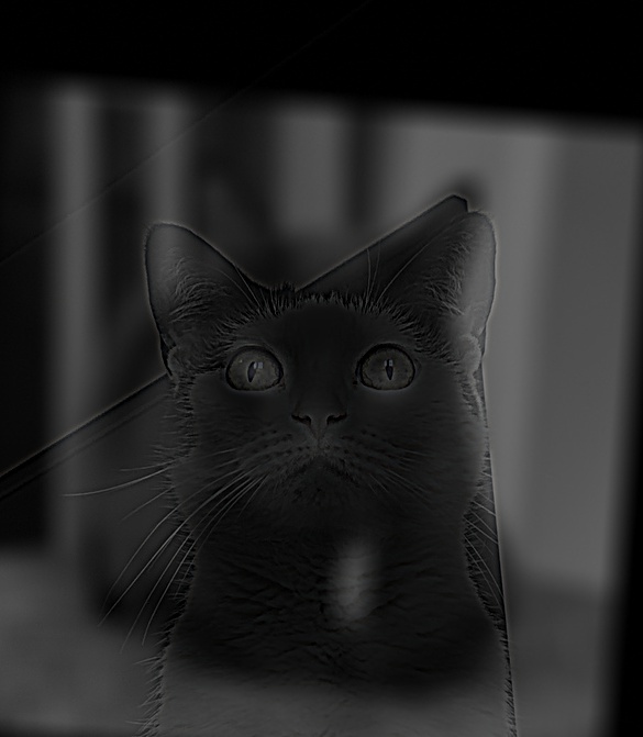
Given the two input images, cat and man, we use the input aligning code.
Man 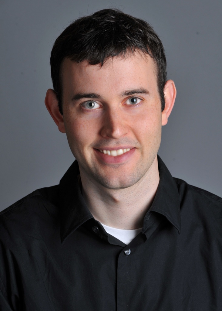
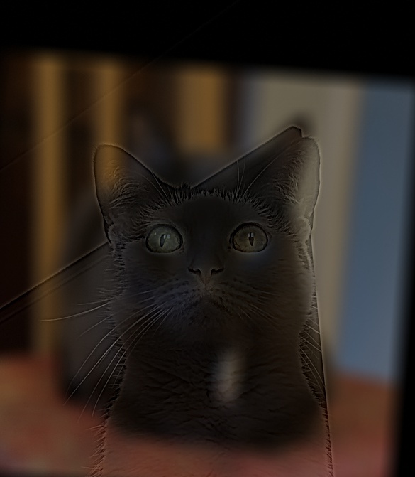
Cat 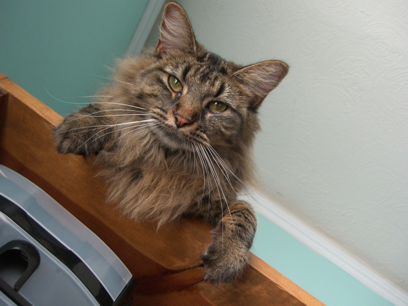
Aligned Man 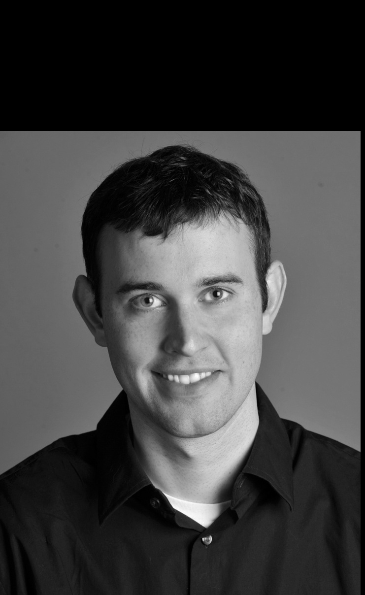
Aligned Cat 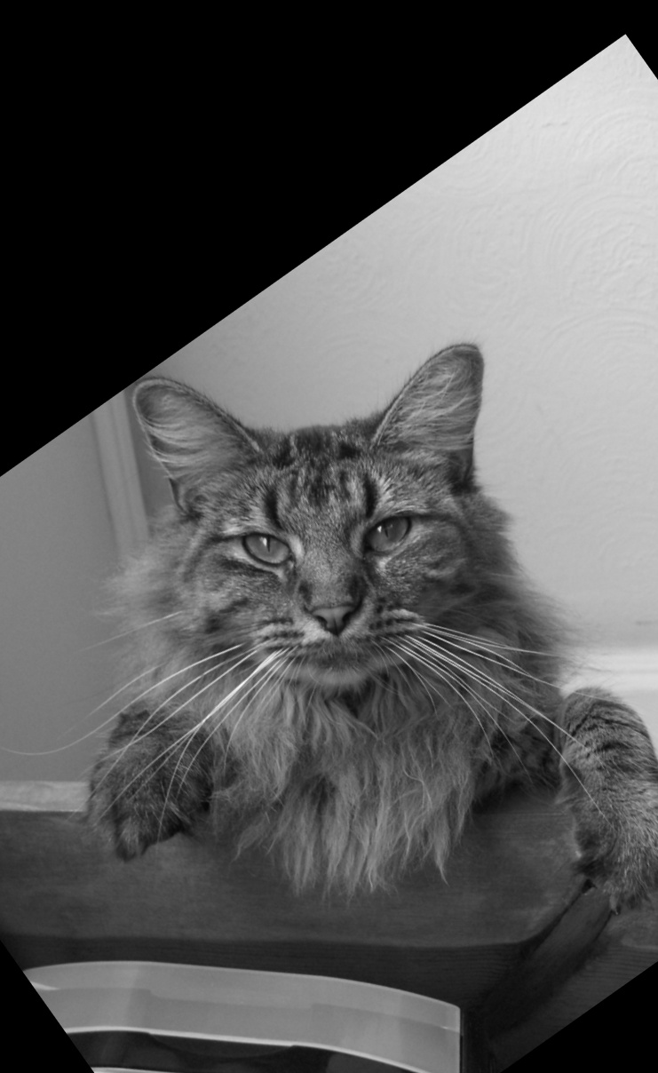
We construct a hybrid image with Gaussian parameters:
sizeL=39, sigmaL=5, sizeH=21, sigmaH=9
LF Man 
HF Cat 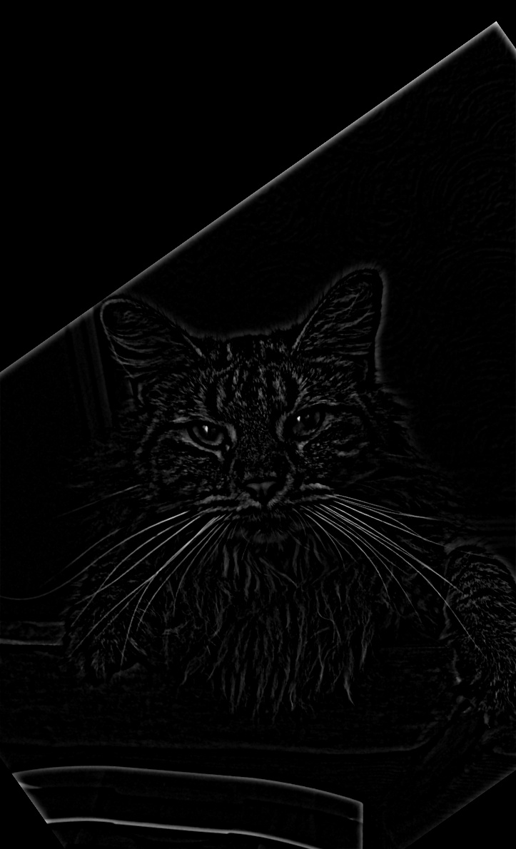
Hybrid 
LF Man (Fourier) 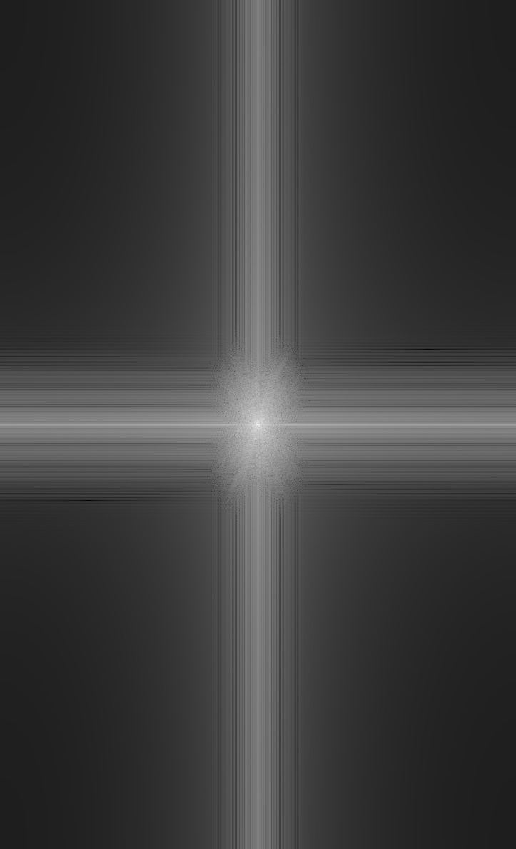
HF Cat (Fourier) 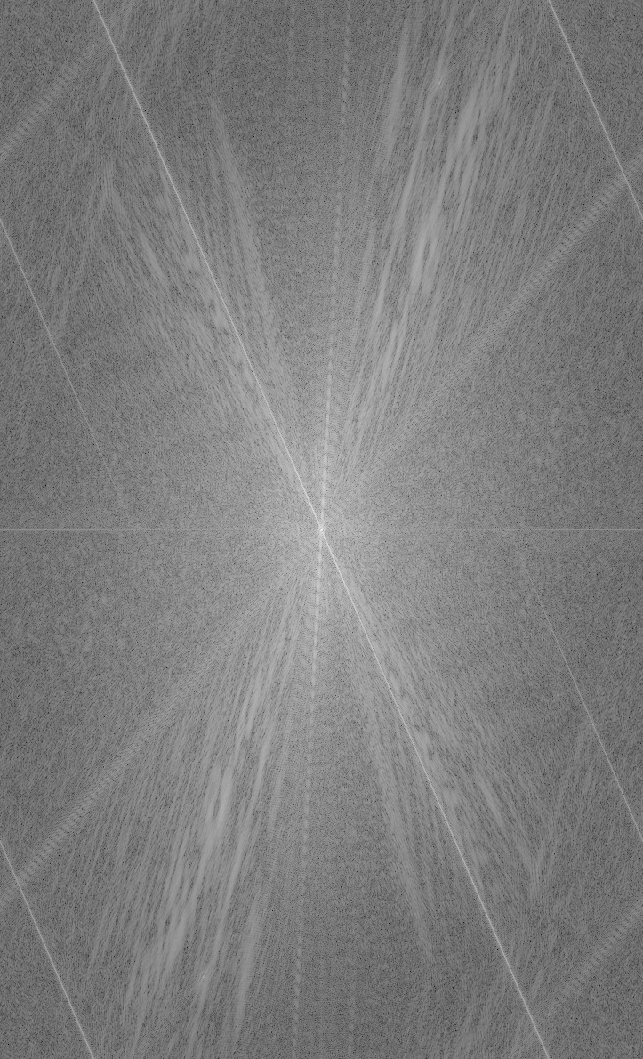
Hybrid (Furrier) 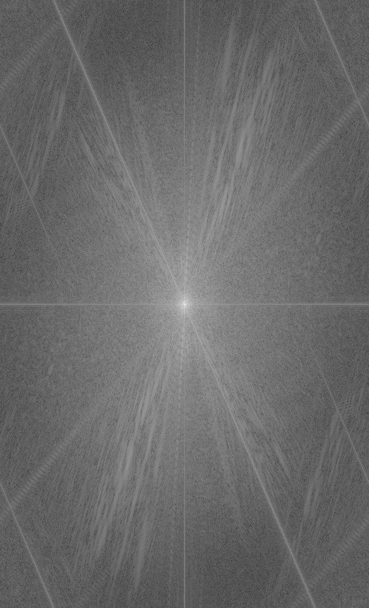
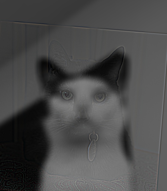
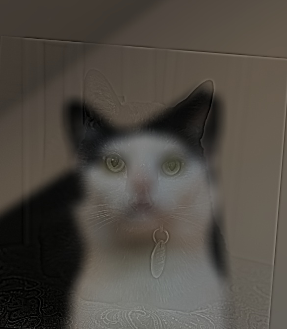
Luna 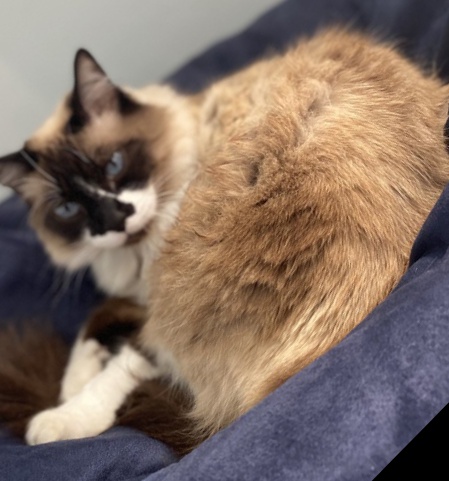
Queen 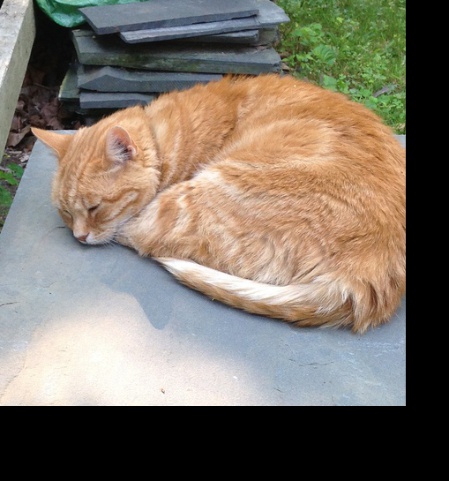
This hybrid image is a failure, as the positions of the cats do not line up. The cats’ bodies are in similar poses, but the heads do not align. Edges from the high-frequency cat are still visible as you move away. Alignment greatly influences the perception of the hybrid image.
sizeL=9, sigmaL=3, sizeH=15, sigmaH=3
LF Cat 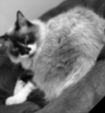
HF Cat 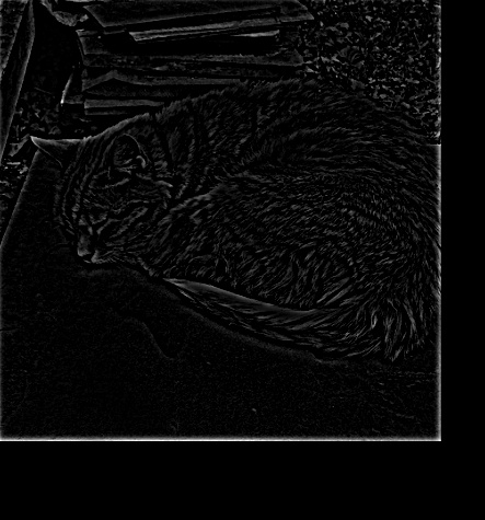
Hybrid 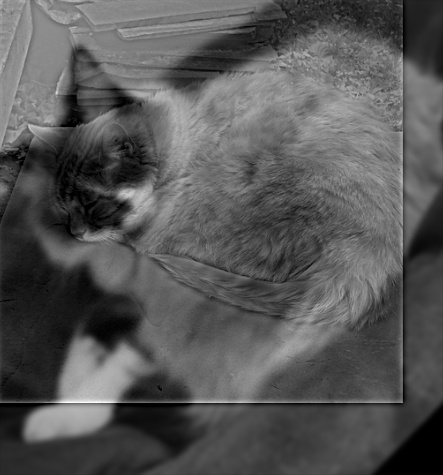
LF Cat (Fourier) 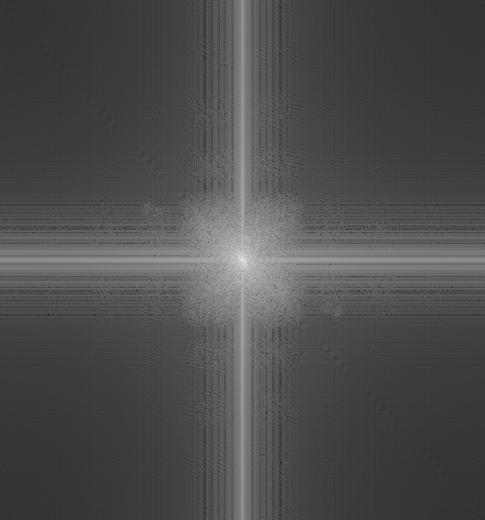
HF Cat (Fourier) 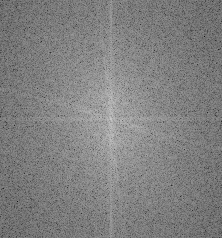
Hybrid (Fourier) 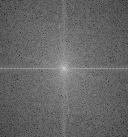
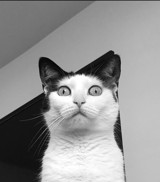
Nocturne 
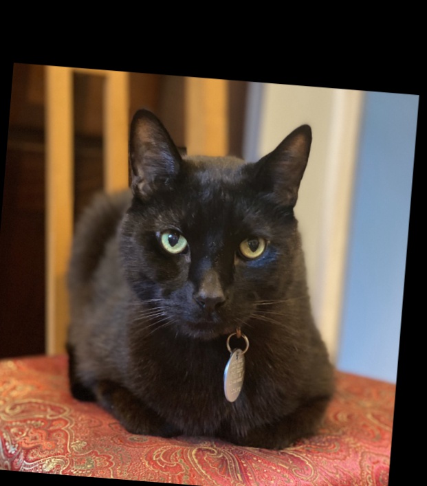
Onyx 
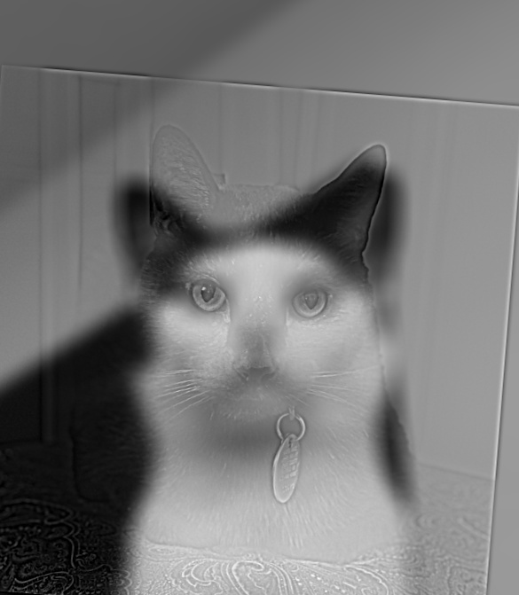
Hybrid BW 
Hybrid Color 
This hybrid image worked out much better. I also liked blurring the frequencies per channel, which seemed to let Onyx’s white face fade into the background. I think both the pose and colorization enhances the perceptual blending of these two cats.
sizeL=30, sigmaL=18, sizeH=11, sigmaH=3
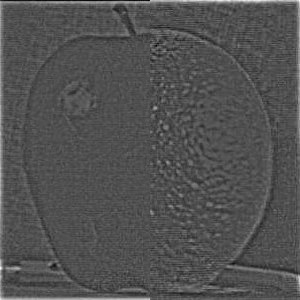
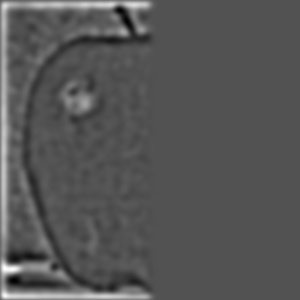
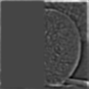
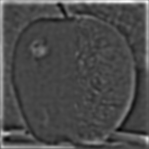
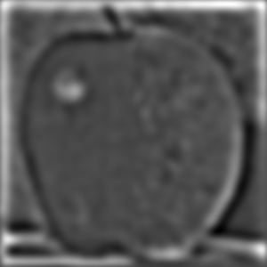
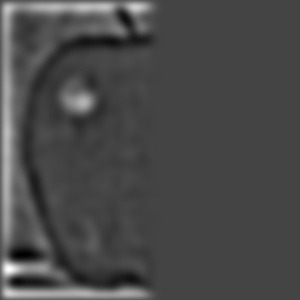
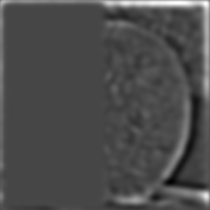
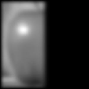
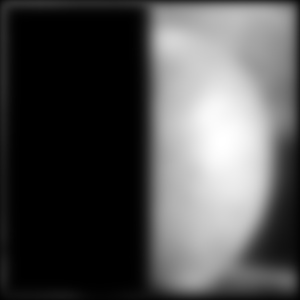
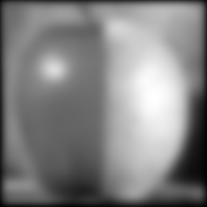
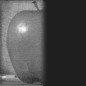
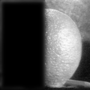
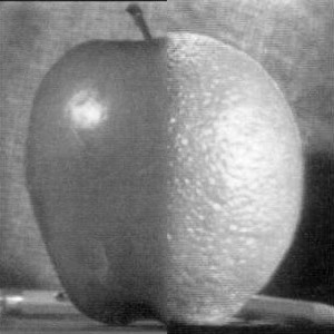
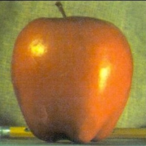
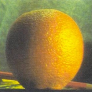
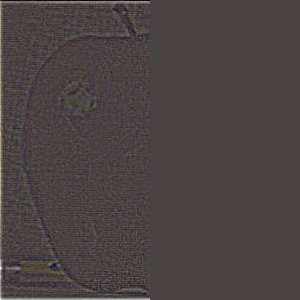
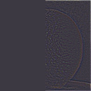
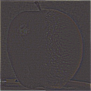
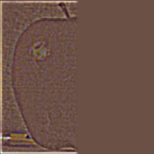
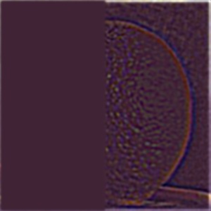
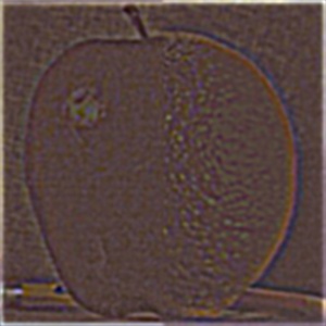
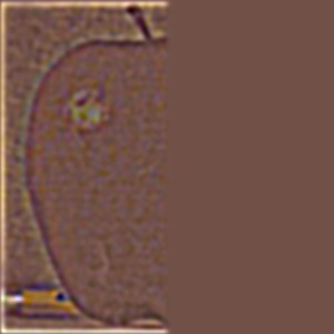
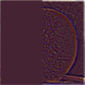
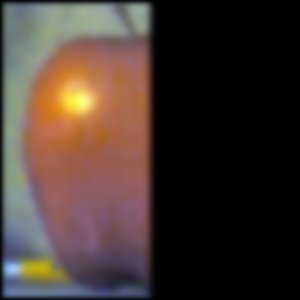
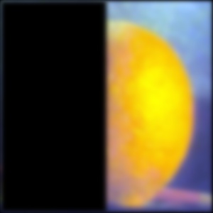
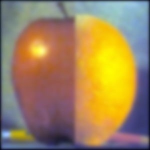
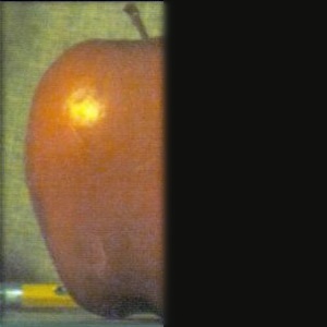
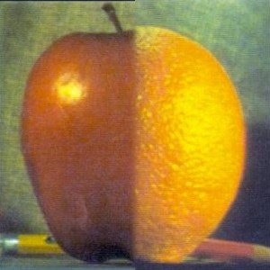
I implemented the Gaussian and Laplacian stacks. For the kernel, I start with a size of 9 and increase it by 9 every deeper level (e.g., 9, 18, 27, …). Recreating the outcomes of Figure 3.42, where the first five rows show the Laplacian detail (levels: 0, 1, 2, 3, 4) with a stack that is 5 deep. The bottom row shows the combined result from all the stacks. The left column shows the apple weighted with the region mask, the middle shows the orange weighted with the region mask (1-R), and the right shows their sum.


In addition to doing the blending per resolution, I also blended the images per color channel. I also increased the stack depth to enhance the blending effect.
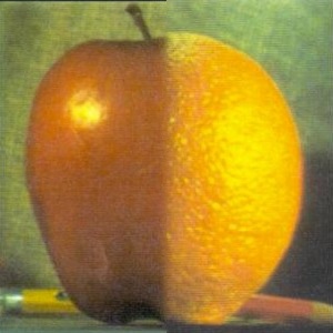
The above blended oraple image was created using 9 levels to smooth the seam. Now I create and visualize the Gaussian region masked images, once again using 5 stack levels (as opposed to 8 for the image above). The final level of the Laplacian stack is the same as the Gaussian stack at that level. Masked and combined images for the apple and orange:
Viewing Normalized Laplacian Stacks (L, R, Blended)
Accumulated Images
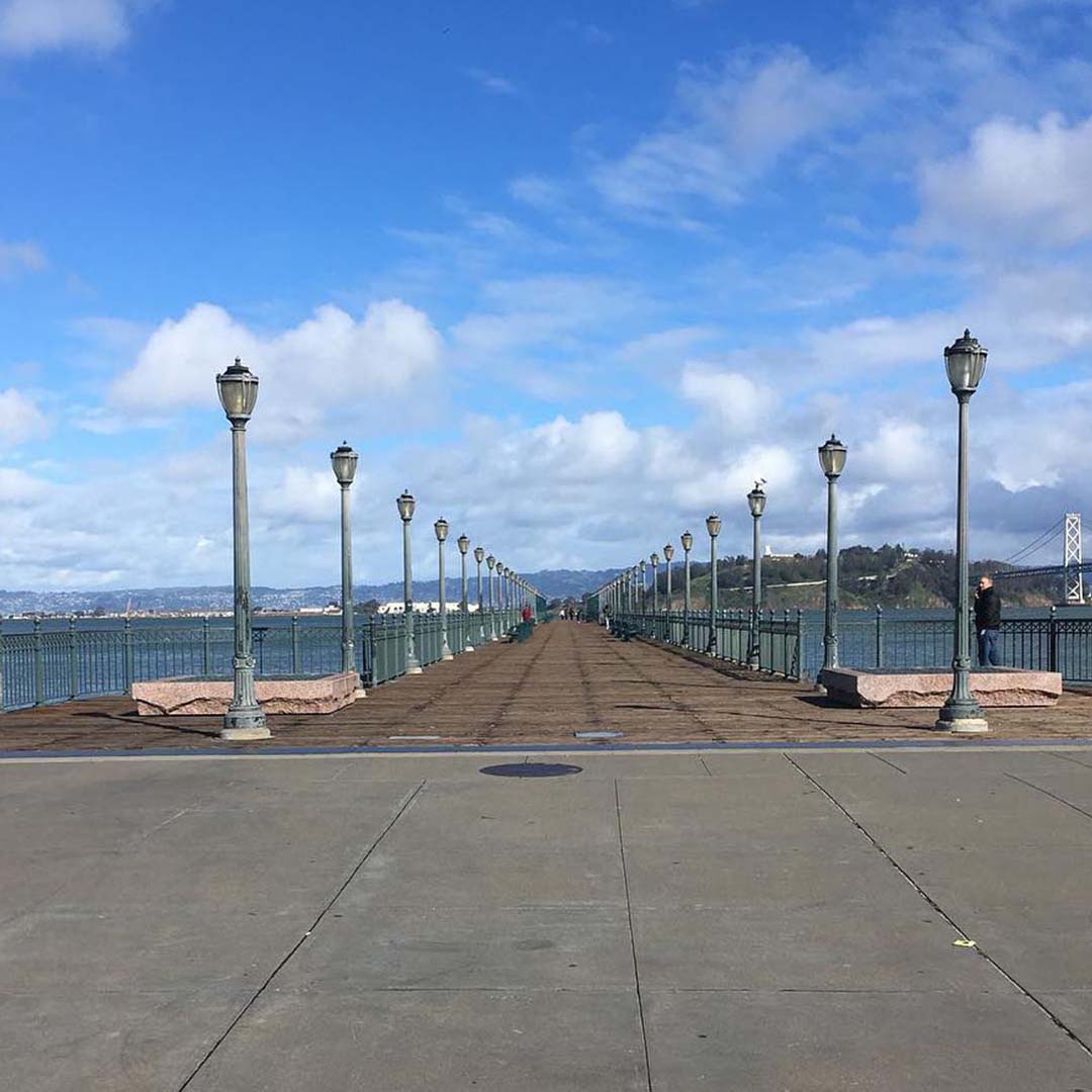
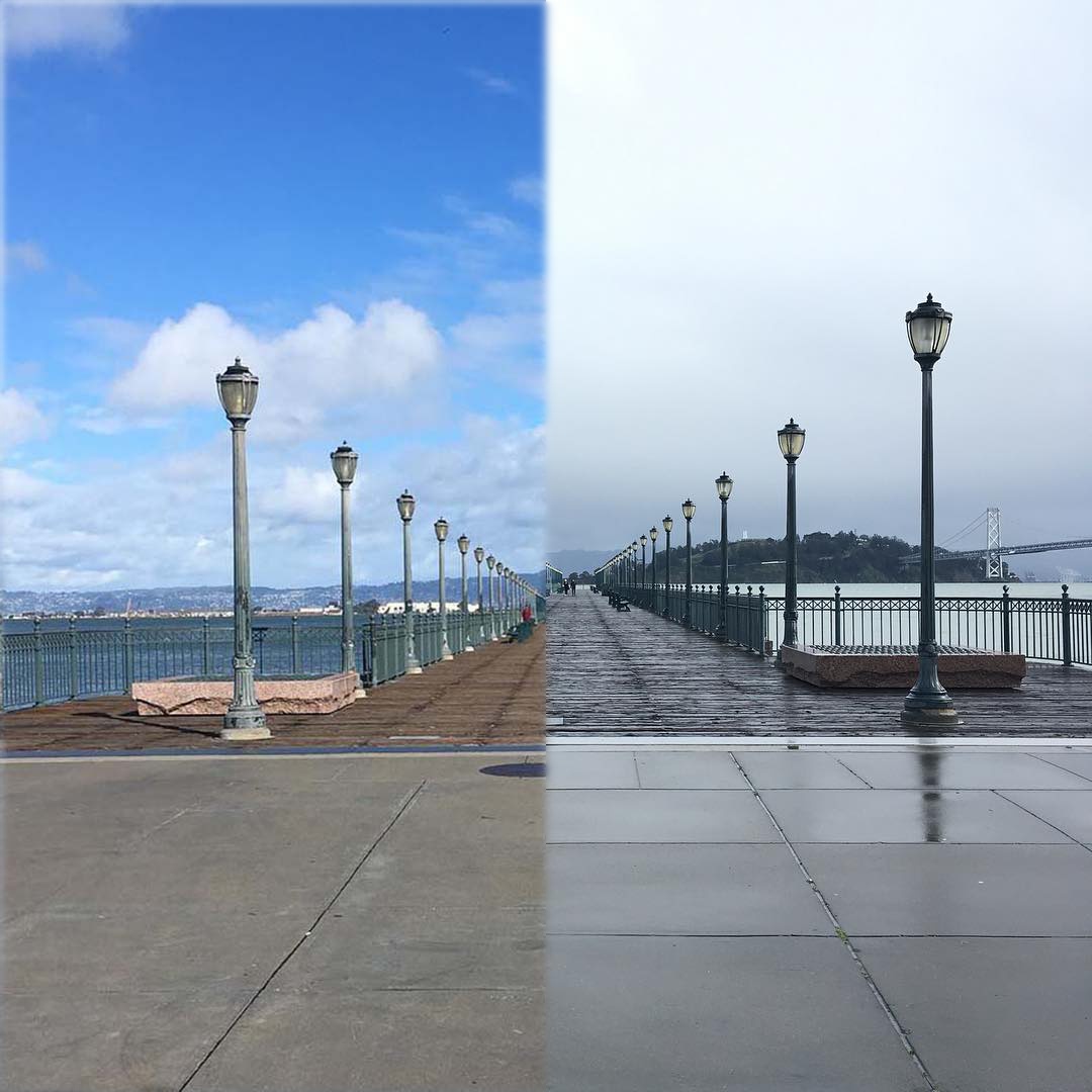
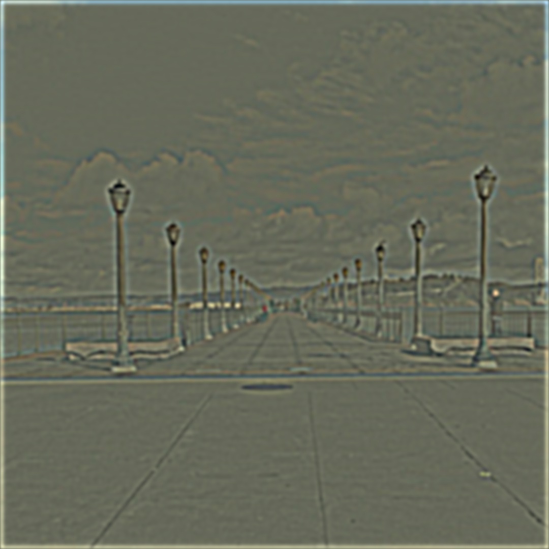
I wanted to blend two pictures I took of the pier in Embarcadero with different weather conditions. Originally I tried making the multi-image blending with the same LR region mask. However the results were subpar due to the images not being vertically aligned.
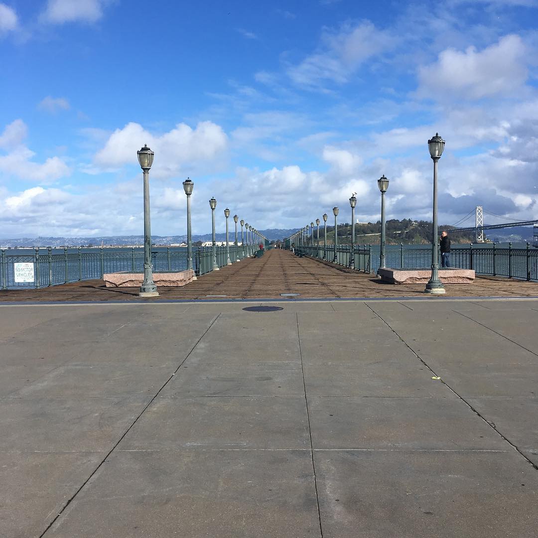
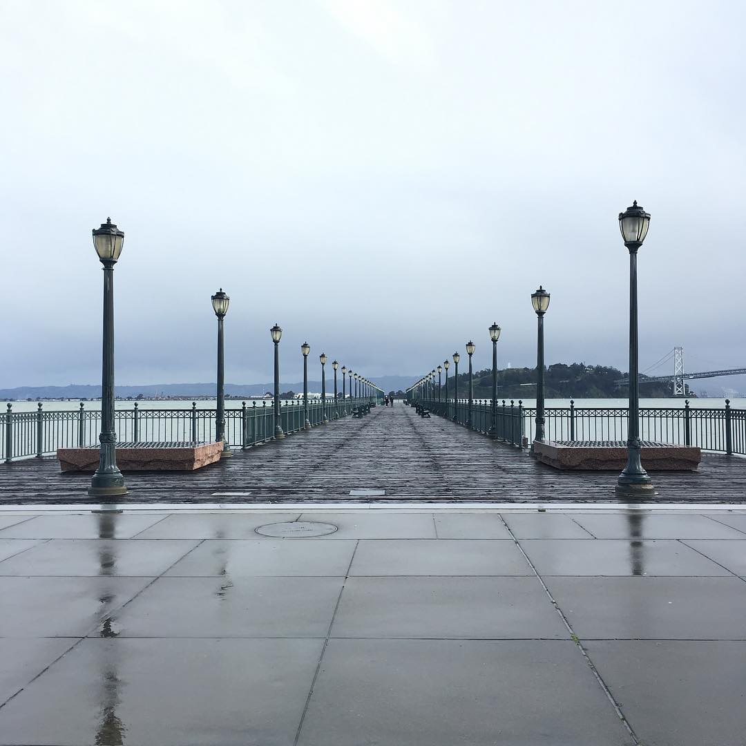
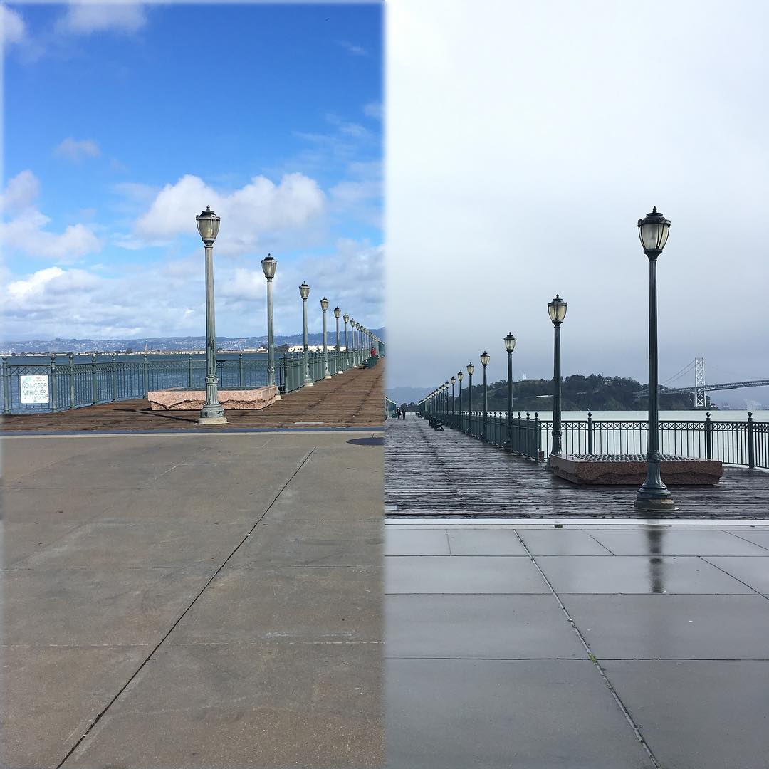
I adjusted the images to be roughly vertically aligned on the docks, then recombined them. There are still some perspective differences that are visible when looking at the lamposts, though. A more complex transform (affine) would be needed to match perspectives.

Full Laplacian Stacks (row 0: “sunny-left”, row 1: “foggy-right”):
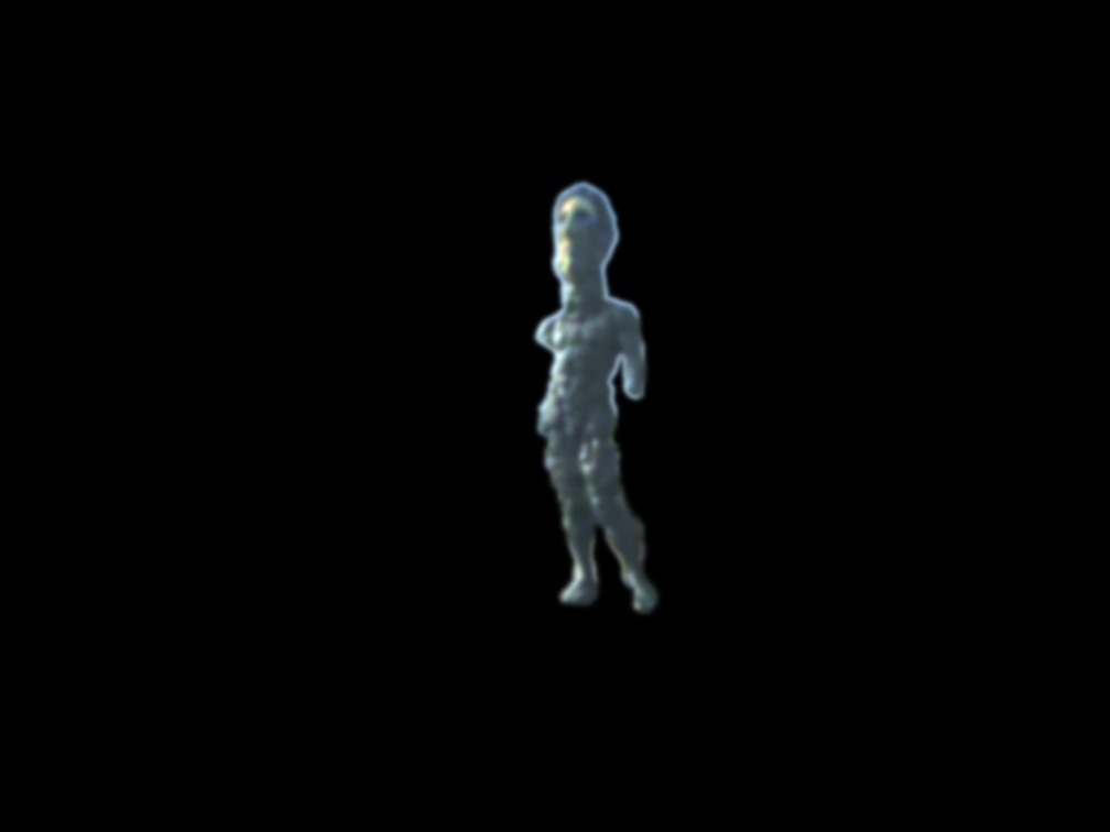
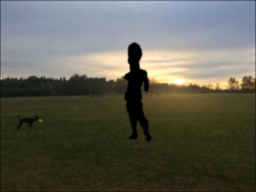
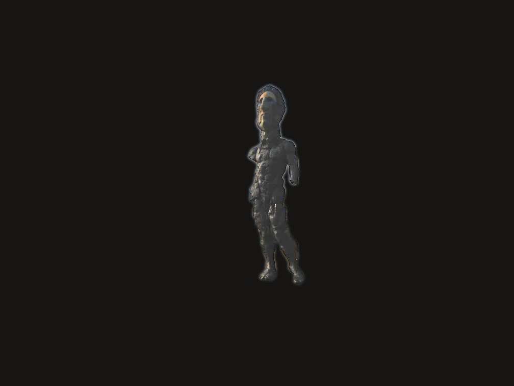
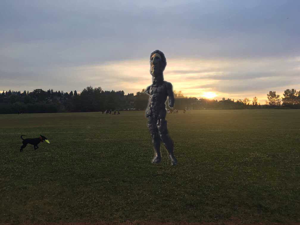
Statues lead such stoic lives. I put this statue on the ultimate frisbee field so it could have some fun. I took these images, then matched their sizes and masked the statue region.
Here is the blended result and normalized Laplacian stacks:


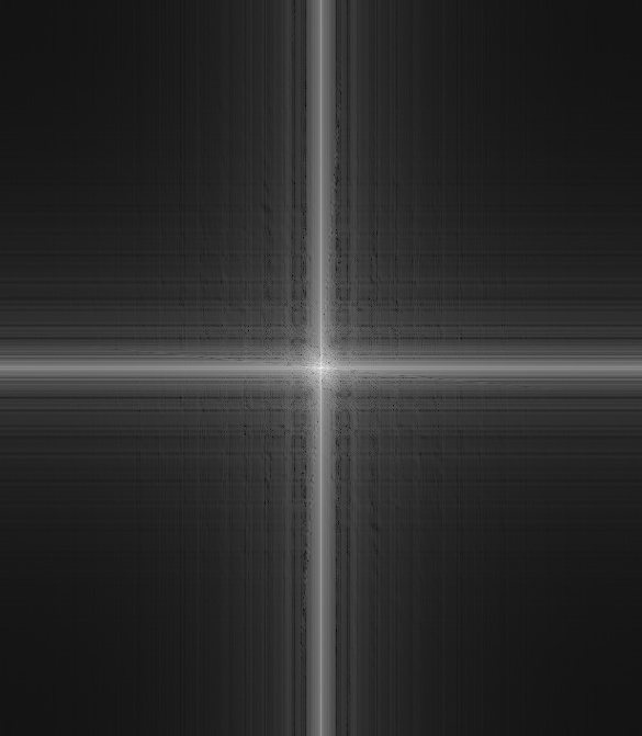
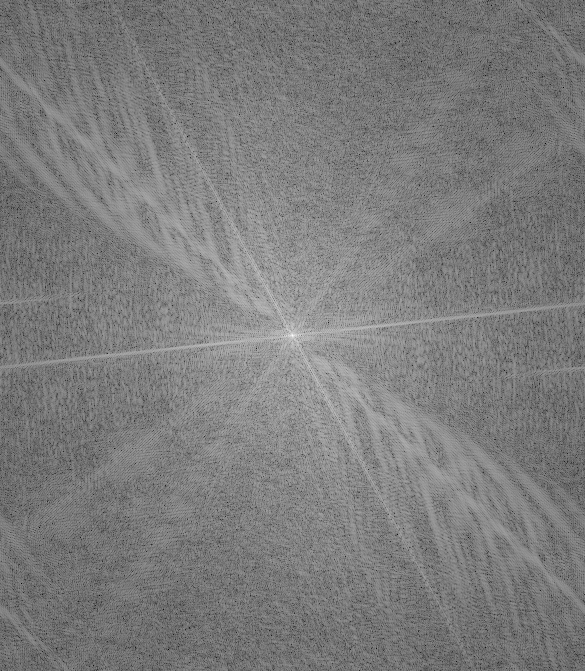
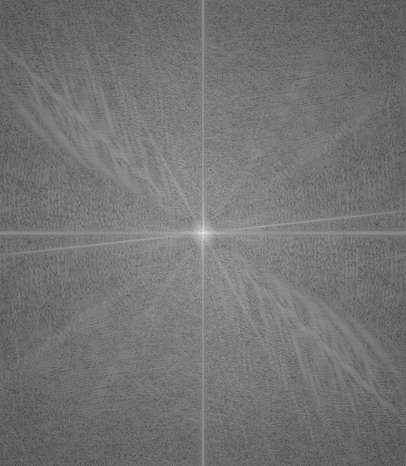
The most interesting thing I learned from this assignment is that you cannot take the Fourier transform of a 3D image. More specifically, it only makes sense to do this transform/visualization on grayscale images, or an images color channels (source). numpy will still happily process this for you given the FFT visualization command from the spec, but it’s hard to discern any sensible information from it. Kind of looks cool though.


Using: np.log(np.abs(np.fft.fftshift(np.fft.fft2(im))))
For this section, I enabled and experimented with mixing the color channels on the images for extra credit. I did this both for the multi-resolution image blending (bw and colored) and hybrid imaging, though I’ll focus on showing color’s effect with hybrid images. In general, human sensitivity to color is lower, so the best target for using color to enhance blending of any type will be in the lower frequency. This is also evident in the JPEG Discrete Cosine Transform transformation which discards high-frequency information like color hue (source). We can run a few experiments to make this difference clearer.
I vary two parameters to generate these images: the image ordering (Onyx/Nocturne vs. Nocturne/Onyx) and color inclusion (none, low-f, high-f, all). More specifically: none means both images are converted to grayscale prior to blending; LF means the lower frequency band image is colored and blended with the grayscale high-frequency band image; HF means the higher frequency band image is colored and blended with the grayscale low-frequency band image; all means two color images are blended (which functionally means they are blended per color channel).
A very interesting takeaway here is that the Color LF and Color All columns look nearly identical. This reinforces the relative decreased human sensitivity to color perception. Basically, humans are not sensitive to high-frequency color information.

Light LF/Dark HF

Dark LF/Light HF

Darker (or more colorful) images should be set in the lower frequency range for better hybrid images as a result. Nocturne is barely visible in any of the Light LF/Dark HF images, even when moving very close to the image. Some images from Dark LF/Light HF to further highlight the importance of ordering/contrast for successful blending:
No Color fails to hide Onyx smoothly, partially due to the sharp edges around the ears which is due to imperfect alignment. Color HF is too good at hiding Onyx, as it darkens the image and makes Onyx barely visible even when closely examing the image. Color LF (and Color All) strike a good balance between these options, blending Onyx and Nocturne the most smoothly, for me. Note: I actually have no cats, though I do like them.