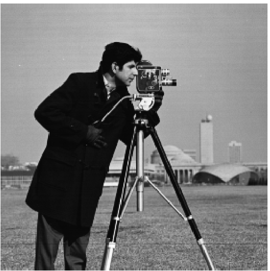
In this part, we would be convolving and filtering using gaussian on the cameraman image
We first initialize the humble finite difference operators d_x and d_y as
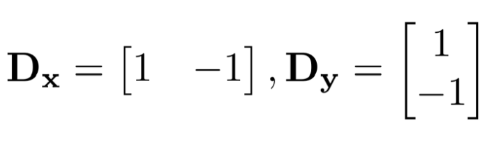
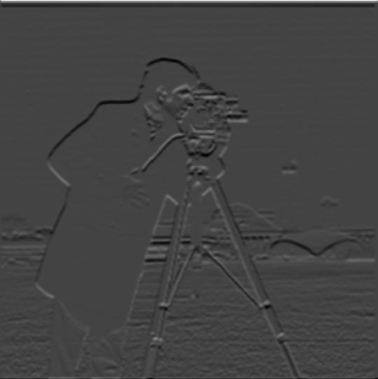
Where we would then convolve the cameraman image with d_x and d_y getting the partial derivative in x and y for the cameraman image
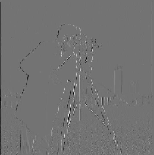
Partial derivative of cameraman in x (partial_x.jpg)
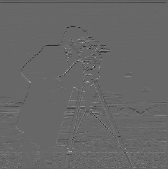
Partial derivative of cameraman in y (partial_y.jpg)
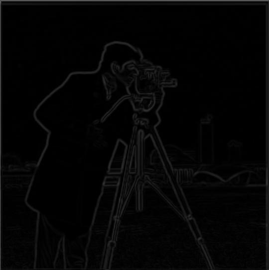
We would then get the gradient magnitude by doing the square root of the sum of the squared partial x and partial y. We would then get this gradient magnitude image
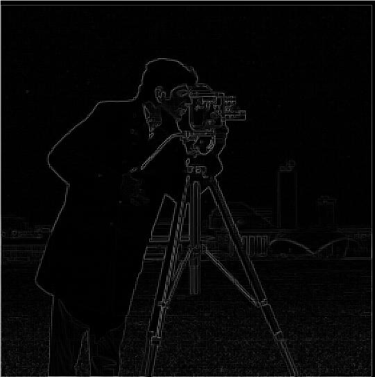
Gradient Magnitude Image (gradient_magnitude.jpg)
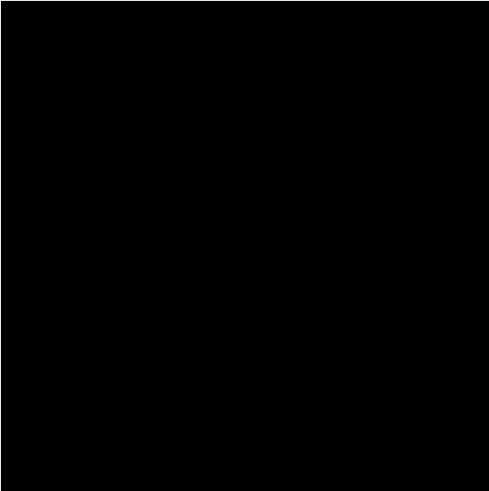
We can then binarize the gradient magnitude image to get the edge image of the cameraman. For this edge image, I used a threshold of 0.25.
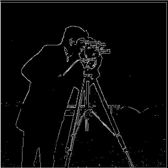
Edge Image with Threshold of 0.25 (binary_gradient.jpg)
In this part, we would be using gaussian as a low pass filter and get the blurry image of the cameraman image
We would first create the Gaussian filter with a sigma of 6 by using cv2.GetGaussianKernel() and take an outer product with its transpose to get the 2D gaussian filter.
After convolving this Gaussian filter with the cameraman image, we get the following blurred image:
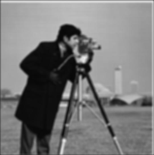
Blurred Image after convolving with Gaussian Filter (blur_img.jpg)
We would then do the same procedures as the previous part (Part 1.1) but convolving the finite difference operators d_x and d_y with the blurred image
The partial derivative of blurred cameraman in x (partial_x_gaussian.jpg)
The partial derivative of blurred cameraman in y (partial_y_gaussian.jpg)
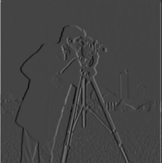
We would then take the gradient magnitude of the blurred image by doing the square root of the sum of squared partial x and partial y. This would give us the gradient magnitude image that has been filtered with the Gaussian filter
Gradient Magnitude of Blurred Cameraman Image (gradient_gaussian_magnitude.jpg)
As we binarize the gradient magnitude of this image, we would get the following edge image:
Edge Image of Gaussian filtered Cameraman Threshold of 0.25(edge_gaussian.jpg)
We could see that there are no significant difference only that it is darker than the previous part.
We would then try to "sharpen" an image by further increasing the intensity of the details of an image. The steps to sharpen an image is as follows:
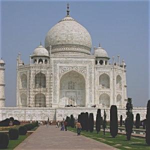
Ex: Taj Mahal Image
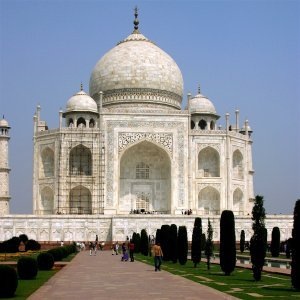
Taj Mahal Original Image (taj.jpg)
Sharpened Taj Mahal, alpha = 0.5, sigma = 3 (taj.jpg_sharpen.jpg)
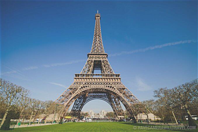
Another sharpened image is the Eiffel Tower Image
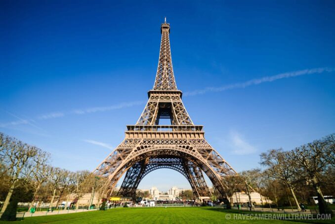
Eiffel Tower Original Image (eiffelTower.jpg)
Sharpened Eiffel Tower , alpha = 0.5, sigma = 3 (eiffelTower.jpg_sharpen.jpg)
Another cool trick we can implement on low and high frequency images are by combining 2 images and merging them into a hybrid image.
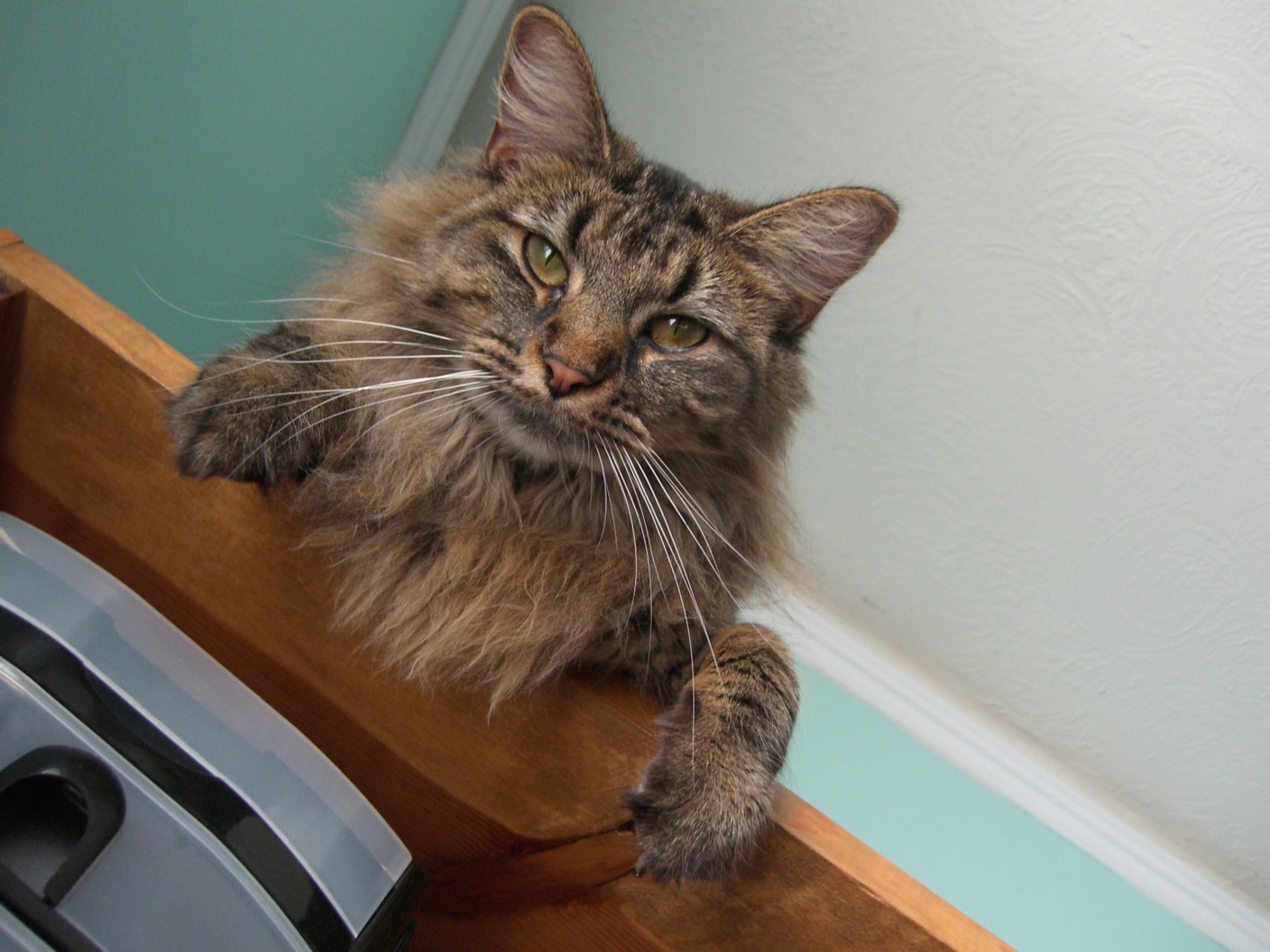
Ex: Derek and his former cat Nutmeg
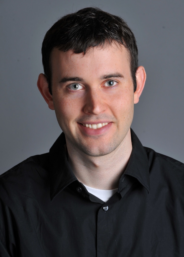
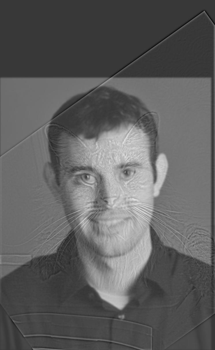
Hybrid Nutmeg and Derek (sigma 3, sigma 5) (nutmeg_derek.jpg)
Ex: Bill Gates and Elon Musk
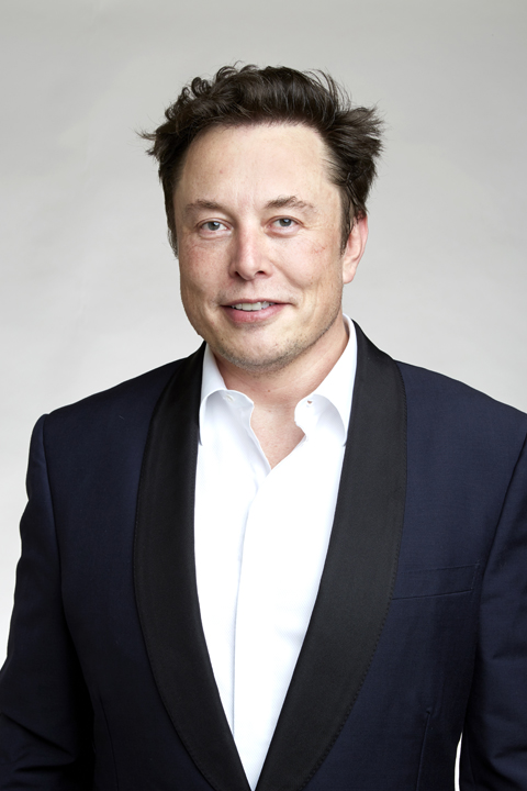
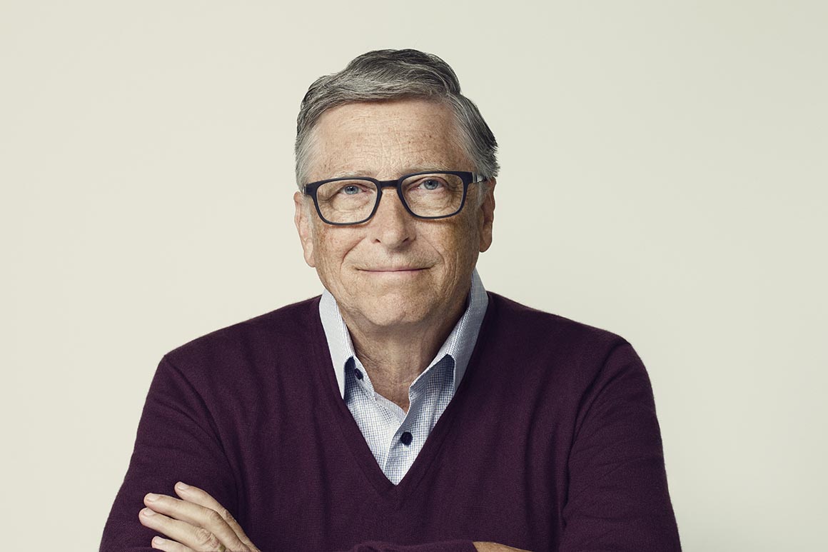
Hybrid Elon Musk and Bill Gates (sigma 3, sigma 5) (gates_musk.jpg)
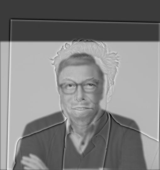
Ex: Lebron James and Stephen Curry
Ex: Lebron James and Stephen Curry
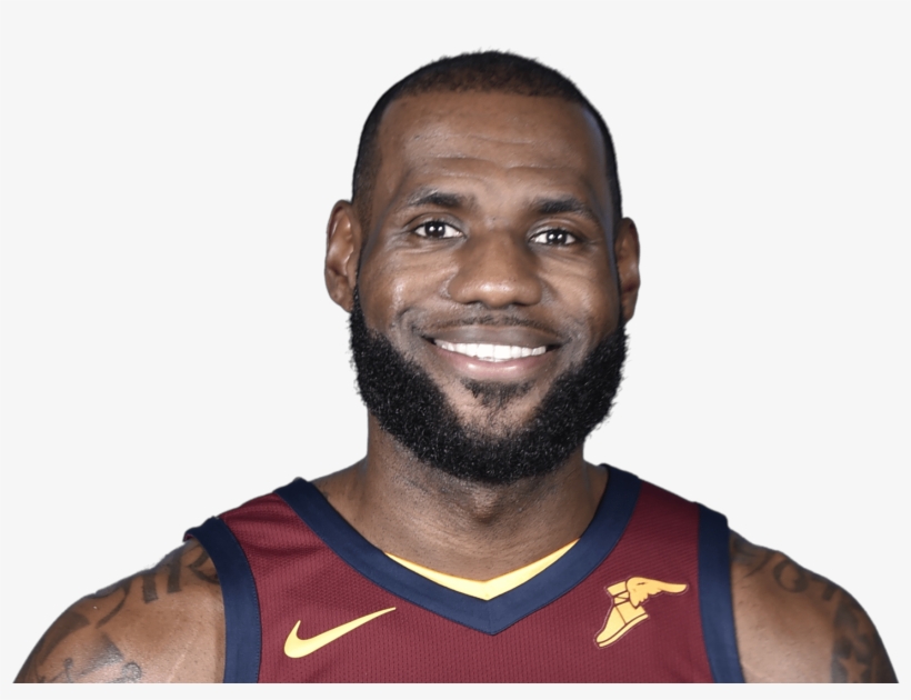
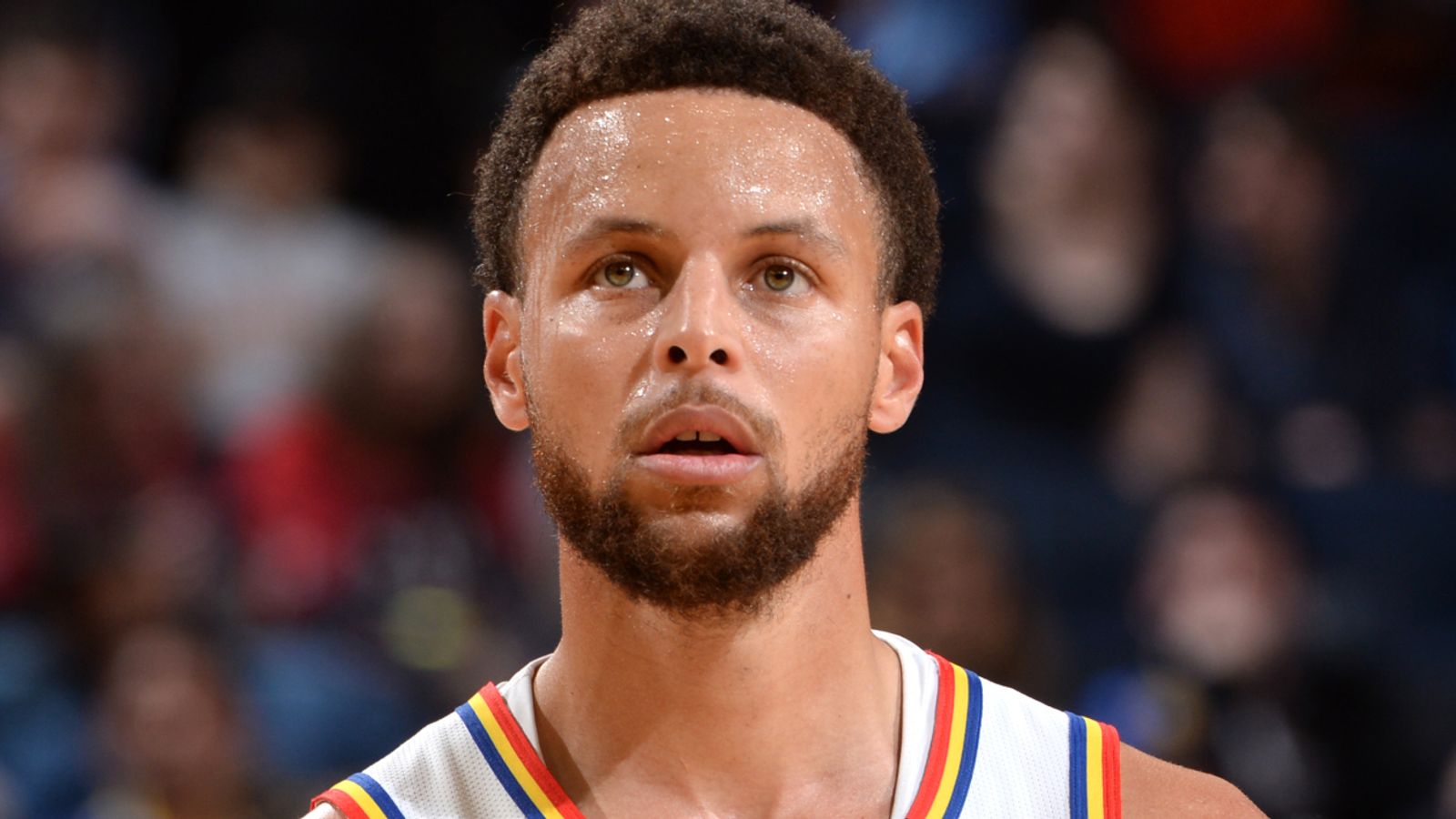
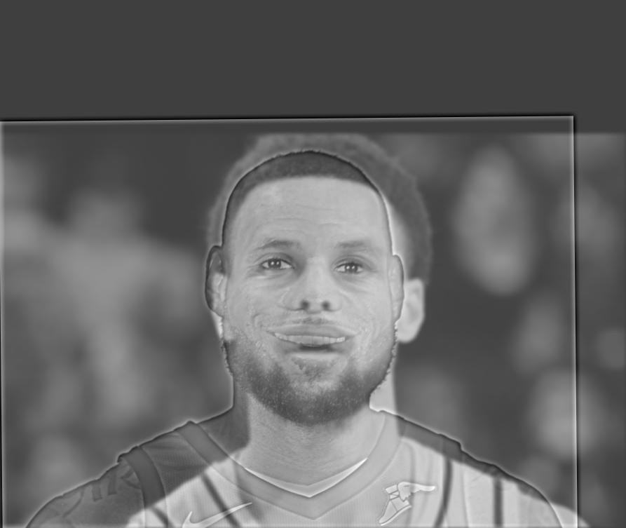
Hybrid Stephen Curry and Lebron James (sigma 3, sigma 5) (curry_lebron.jpg)
We implement the Gaussian Stack which is the gaussian filter for increasing sigma of the original image. In this project, each stack would be twice the sigma of the previous stack (ex: 2, 4, 8, 16, 32)
From this Gaussian Stack, we can get the Laplacian Stack which is just the difference between each stack. And that the last level of the Laplacian Stack is just the last level of the Gaussian Stack.
An implementation of the Gaussian and Laplacian Stack could be seen at the next part (Part 2.4)
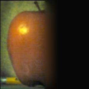
In this part, we would be blending together an apple image and orange image into a oraple:
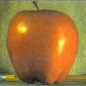
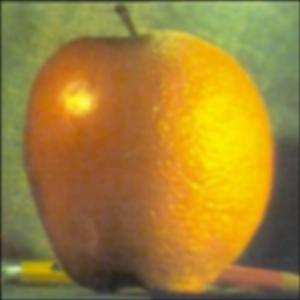
Apple Image (apple.jpeg)
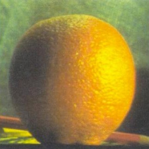
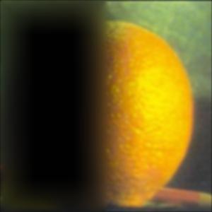
Orange Image (orange.jpeg)
In which we would be creating the Gaussian and Laplacian Stack from Part 2.3 for each of the images.
We would also create a mask matrix (ex: half left is all 1 and half right is all 0). Which would be used to blend the laplacian images for a better transition
For each Gaussian and Laplacian Stack we would also convolve the Gaussian filter on to the mask
We would then get the level's blended image by applying the formula: blended_image = (filtered_mask laplacian_image_1) + ((1 - filtered_mask) laplacian_image_2)
And we would then sum up all the blended image of each laplacian level to get a resulting image.
Ex: Oraple
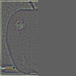
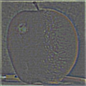
Apple Laplacian Level 1 (sigma 2)(apple.jpeg_2_laplace.jpg)
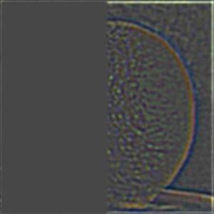
Orange Laplacian Level 1 (sigma 2)(orange.jpeg_2_laplace.jpg)
Combined Oraple Level 1 (sigma 2)(combined_2_laplace.jpg)
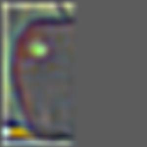
Apple Laplacian Level 3 (sigma 8)(apple.jpeg_8_laplace.jpg)
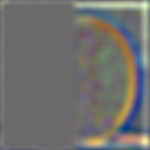
Orange Laplacian Level 3 (sigma 8)(orange.jpeg_8_laplace.jpg)
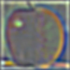
Combined Oraple Level 3 (sigma 8)(combined_8_laplace.jpg)
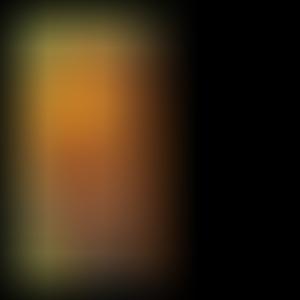
Apple Laplacian Level 5 (sigma 32)(apple.jpeg_32_laplace.jpg)
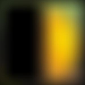
Orange Laplacian Level 5 (sigma 32)(orange.jpeg_32_laplace.jpg)
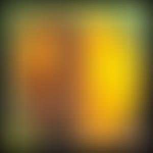
Combined Oraple Level 5 (sigma 32)(combined_32_laplace.jpg)
Total Laplacian Apple (total_laplace_image1.jpg)
Total Laplacian Orange (total_laplace_image2.jpg)
Blended Oraple (result.jpg)