Filters
Part 1.1: Finite Difference Operator
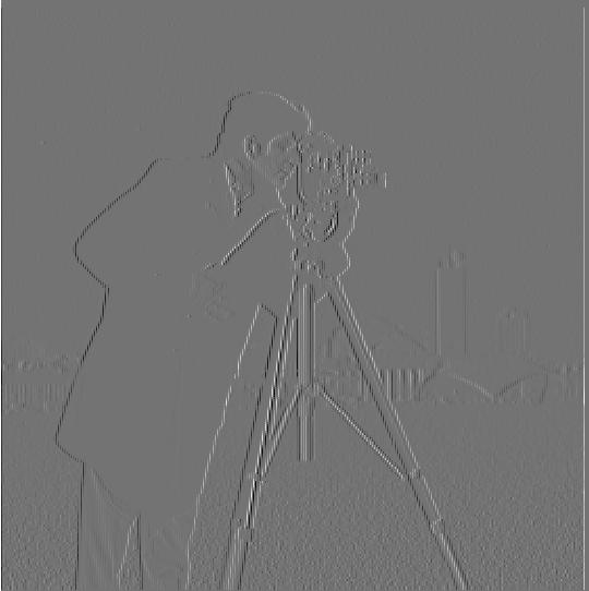
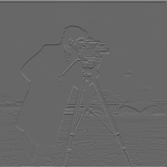
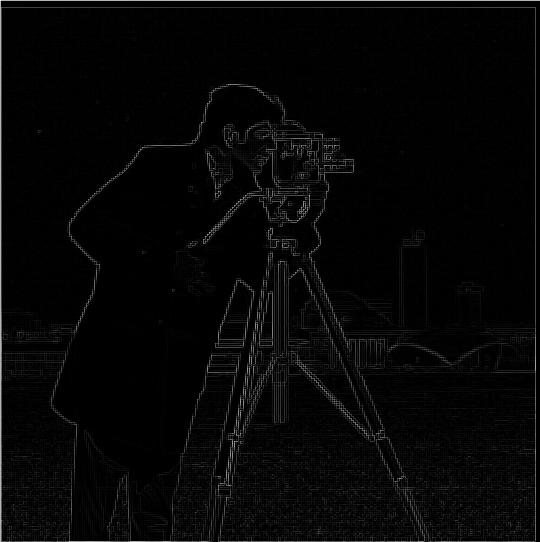
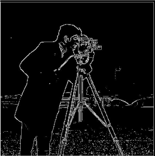
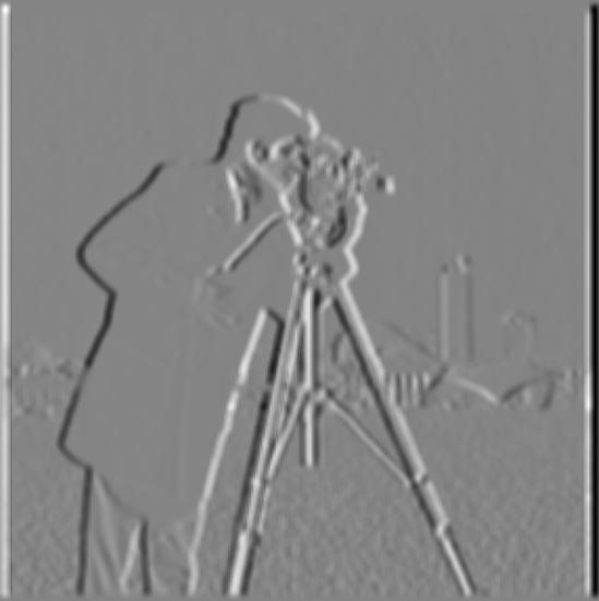
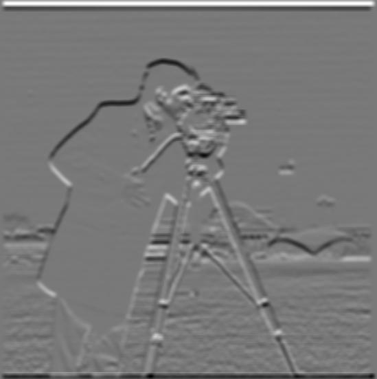
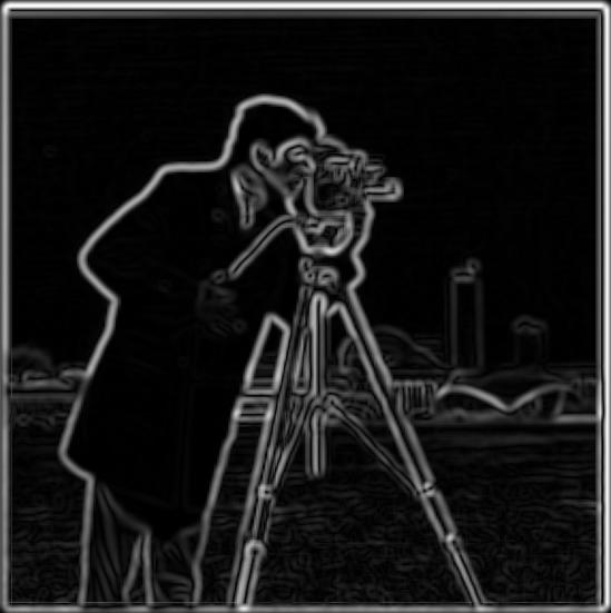
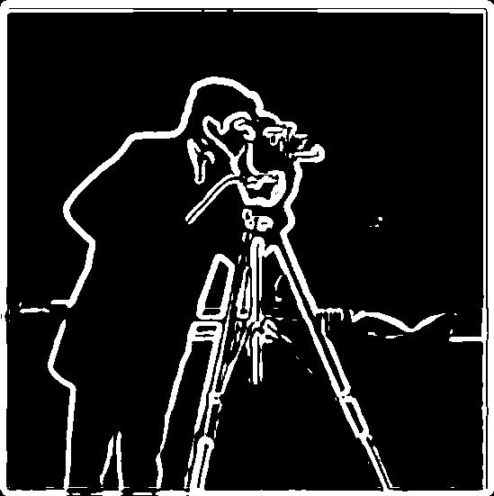
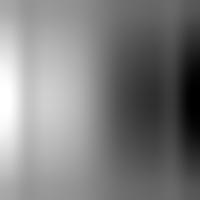
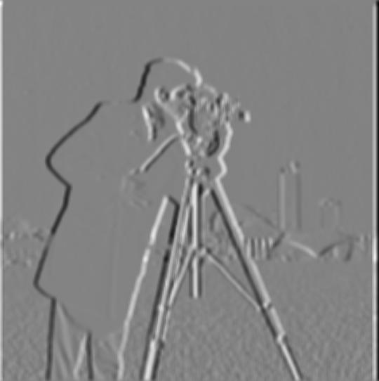
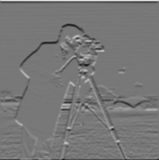
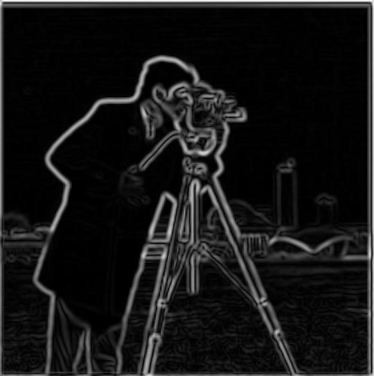
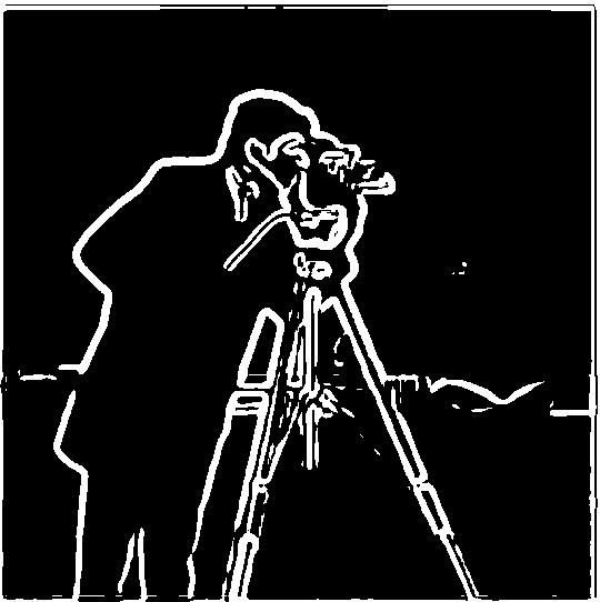
Shown below are the partial derivatives, the gradient magnitude, and binarized gradient magnitude images of a cameraman. To compute and visualize the gradient magnitude, we can use the L2 norm of the gradient vector: $$ \sqrt{(\frac{df}{dx})^2 + (\frac{df}{dy})^2} $$
Part 1.2: Derivative of Gaussian (DoG)
After convolving the original image with a 10 x 10 Gaussian filter with standard deviation 3, the binarized grad norm has much smoother results as opposed to the noisy results shown in the previous section. This is due to the Gaussian filter removing the high frequency image features that contribute to this noise.
Convolving the Gaussian features with the finite difference operator for D_x and D_y first and then convolving the raw (unblurred) cameraman image with those DoG filters yields the same effect.

Frequencies
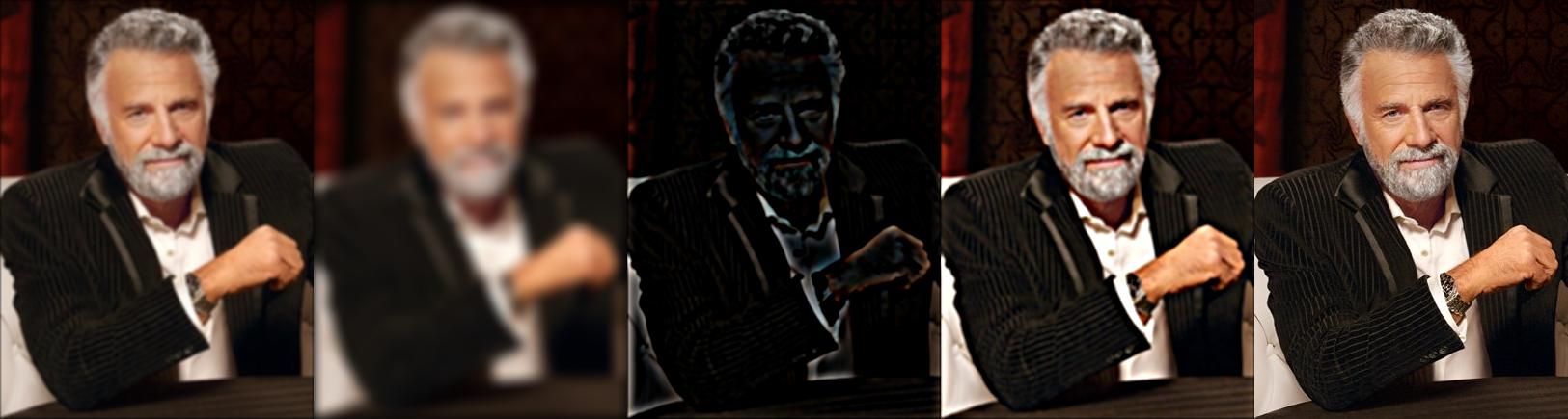
Part 2.1: Image Sharpening
Using the unsharp masking technique, we can produce "sharper" images by amplifying the high frequency signals in the image features. This is accomplished with a 21 x 21 Gaussian filter with standard deviation 7 (for all images shown below), blurring the
initial image, subtracting the blurred from the initial, and then adding the difference multiplied by an alpha coefficient back to the original image. This can also be understood as convolve(f, (1 + alpha) * unit_impulse - alpha * gaussian).
We also clip pixel intensities to a [0, 1] range to prevent numerical overflow/underflow issues when rendering.
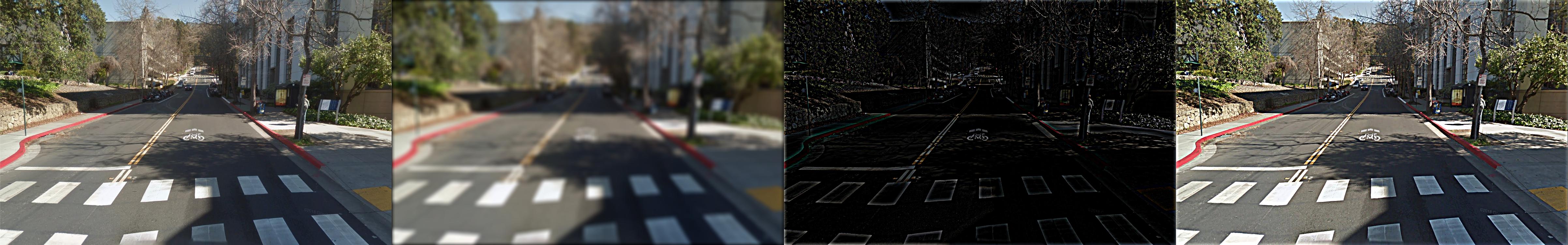
This effect does not work when attempting to recover sharper features from an already blurred image, like in the example below. This is because the Gaussian filter loses information and the high frequency features present in the blurred copy below are not enough to recover the high frequency features in the original (sharper) image.
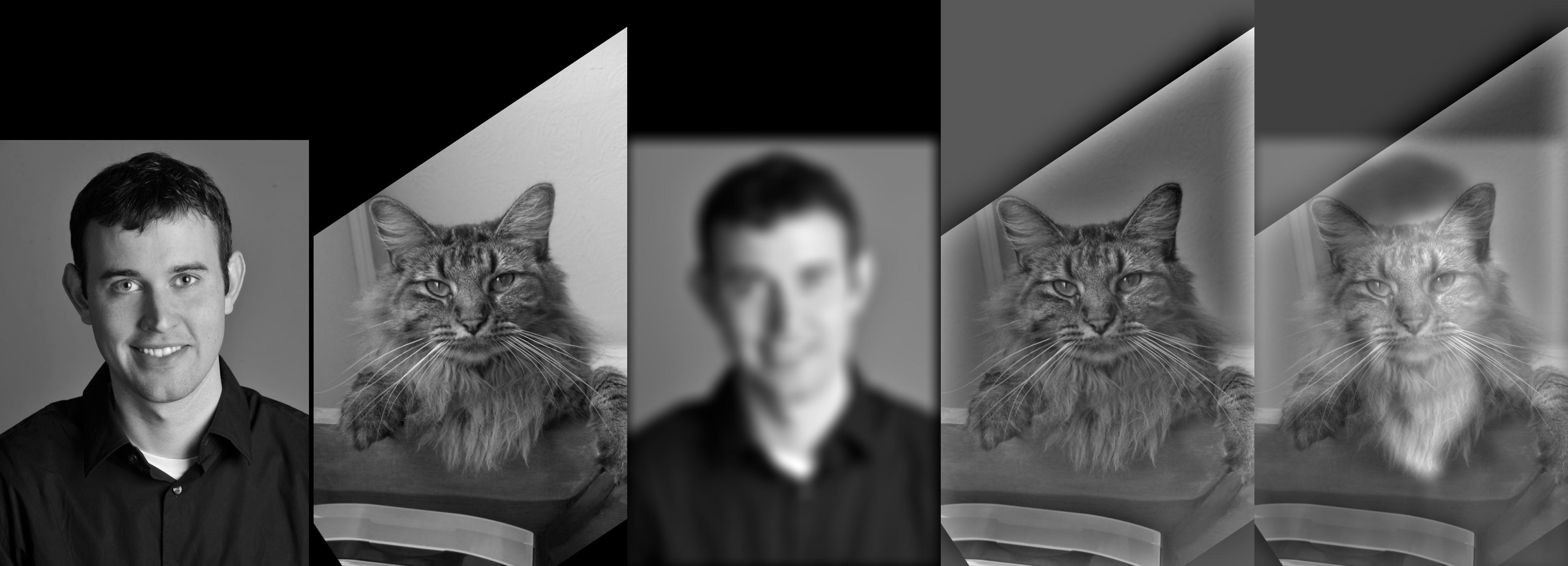
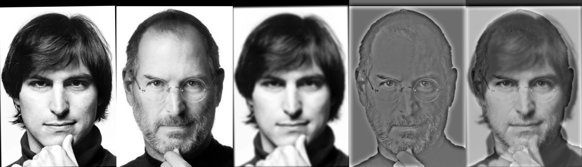
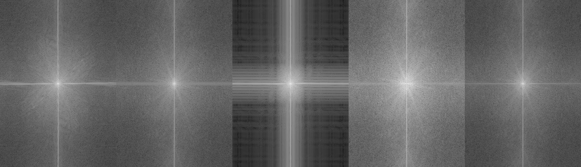
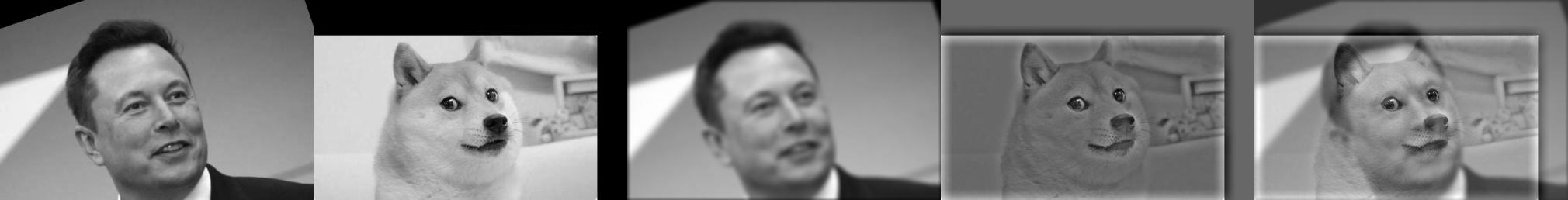
Part 2.2: Hybrid Images
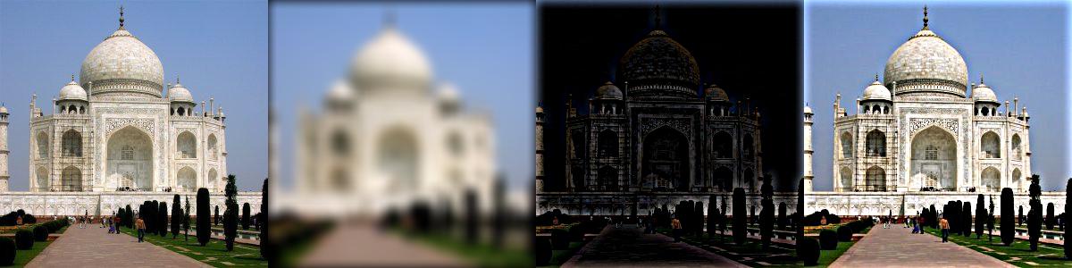
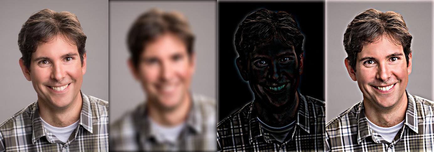
To produce hybrid versions of two images such that one image is visible from a distance and the other image is visible close to the viewer, we blend together images by averaging a low pass filtered image (Gaussian blur) and a high pass filtered image (Gaussian blur subtracted from the original image). This gives the perceptual effect of there being multiple images at various distances due to the Campbell-Robson contrast sensitivity curve.
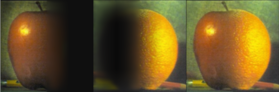
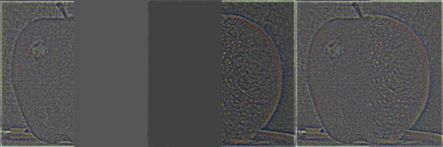
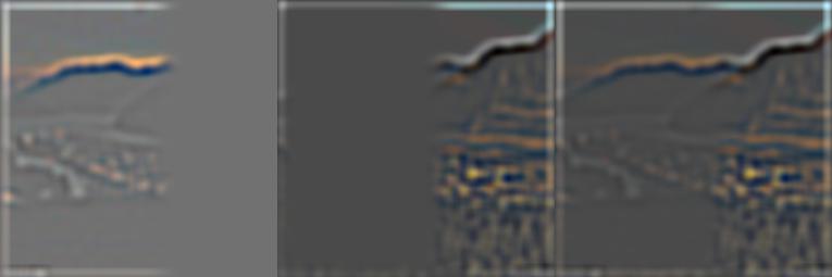
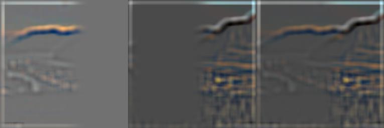
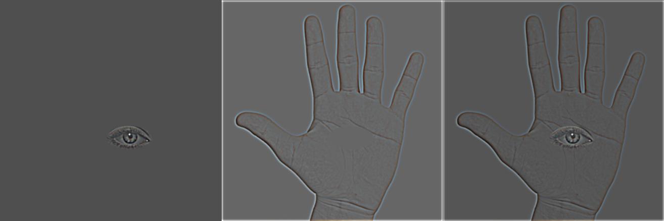
Part 2.3: Gaussian and Laplacian Stacks
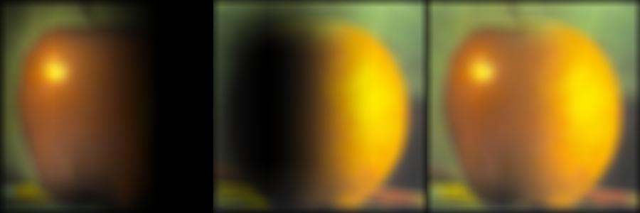
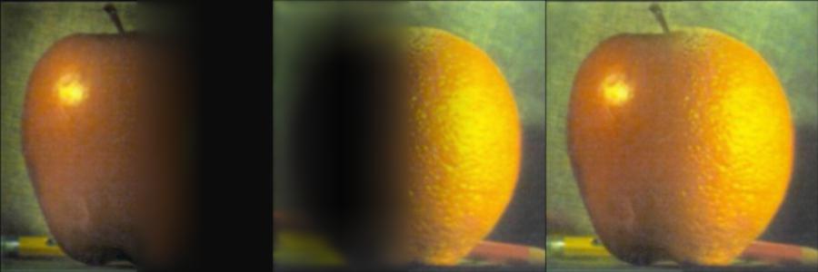
To allow for multiresolution blending, we implement Gaussian and Laplacian stacks. The Gaussian stack is implemented by convolving an input image with Gaussian filters of several different standard deviations down the stack. The Laplacian stack is implemented by subtracting intermediate layers of the Gaussian stack, with the final layer of the Laplacian stack being equal to the final layer of the corresponding Gaussian stack. In all experiments, 5-layer deep stacks are used. RGB images are convolved with Gaussian filters by convolving the Gaussian filter along each color dimension and then concatenating the blurred outputs channel-wise to produce the final blurred RGB image.
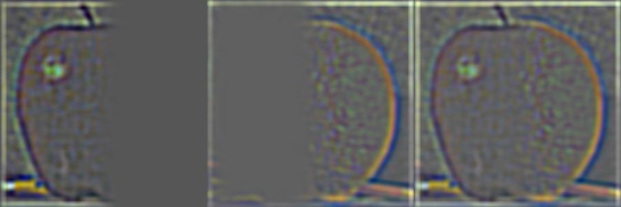
Below we can see the Laplacian stacks for an apple and orange, with each layer in the stack blended with a mask. The mask is used is a step function with the left half set to 1 and the right half set to 0. A Gaussian stack for the mask is generated and each layer in the Gaussian stack of the mask is used to blend the Laplacian stacks at the corresponding level to produce the final Laplacian stack. The final Laplacian stack is used to generate the final blended image by summing all levels in the stack into a single image.
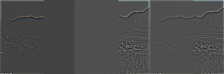
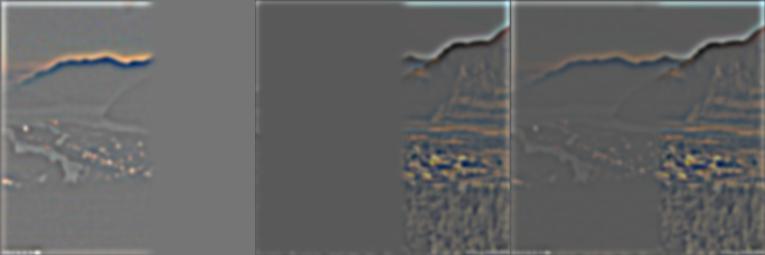
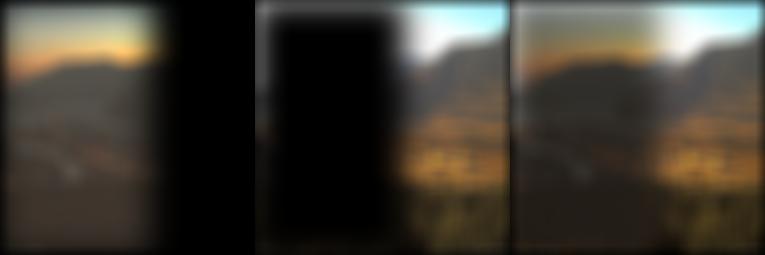
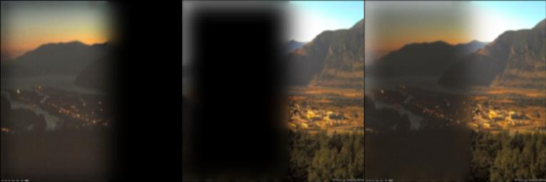
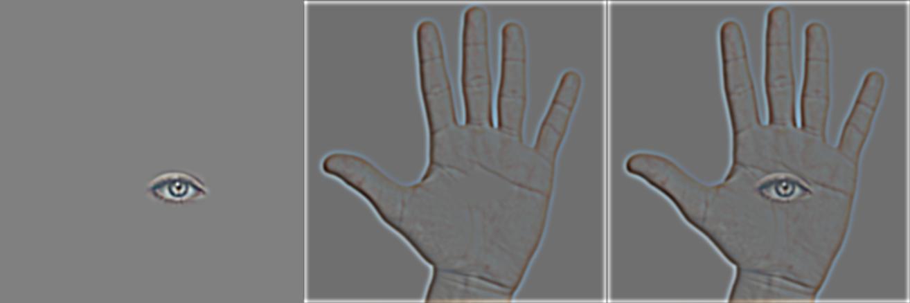
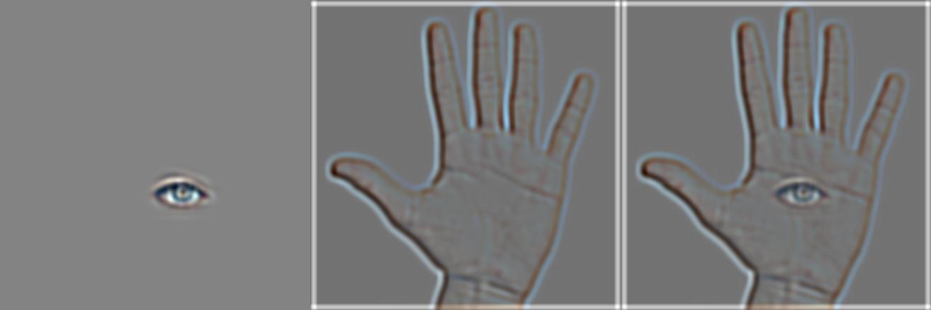
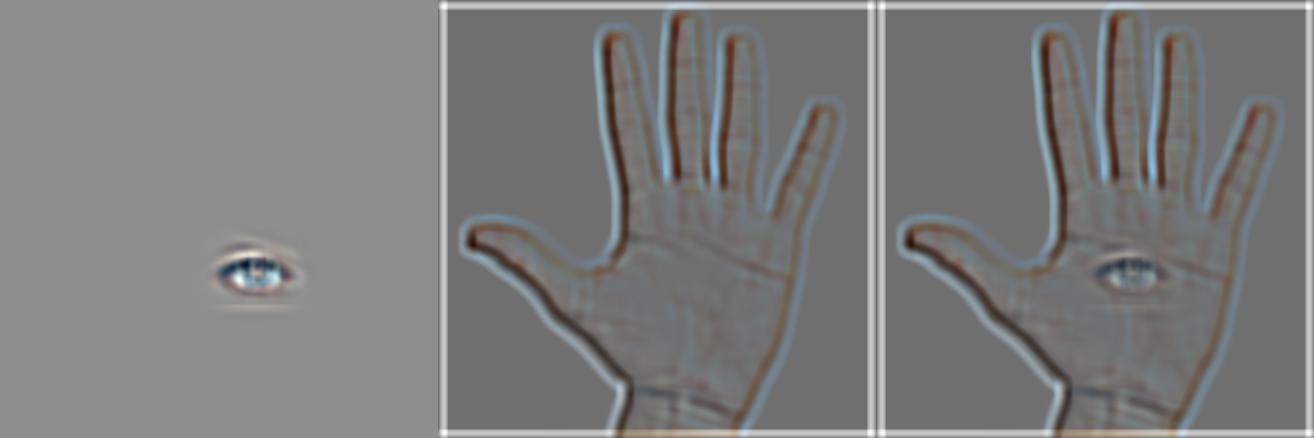
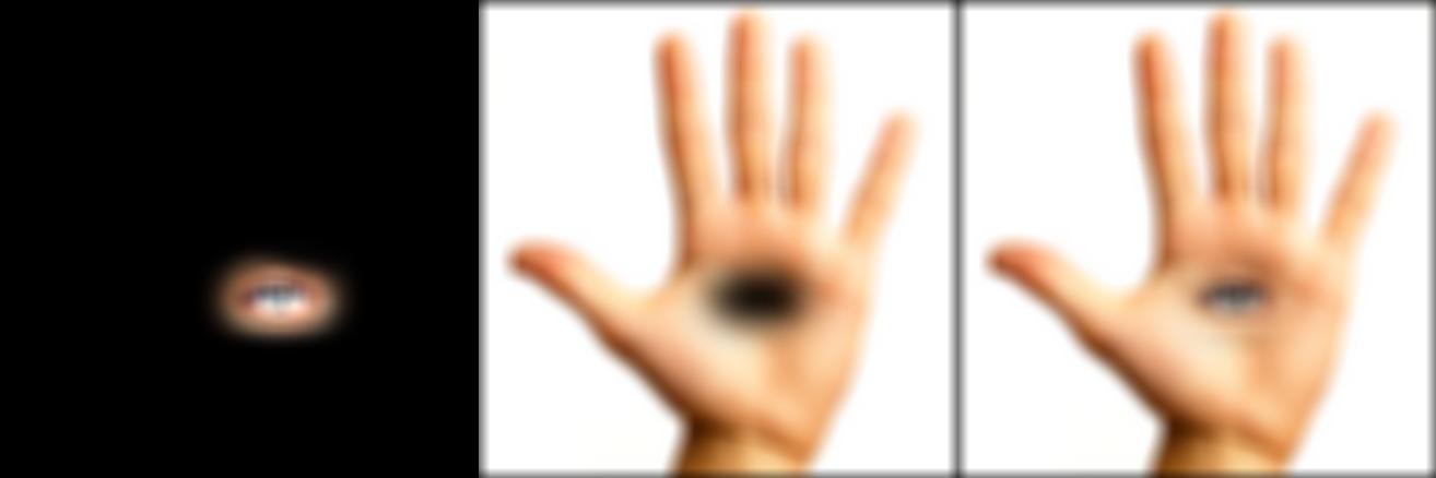
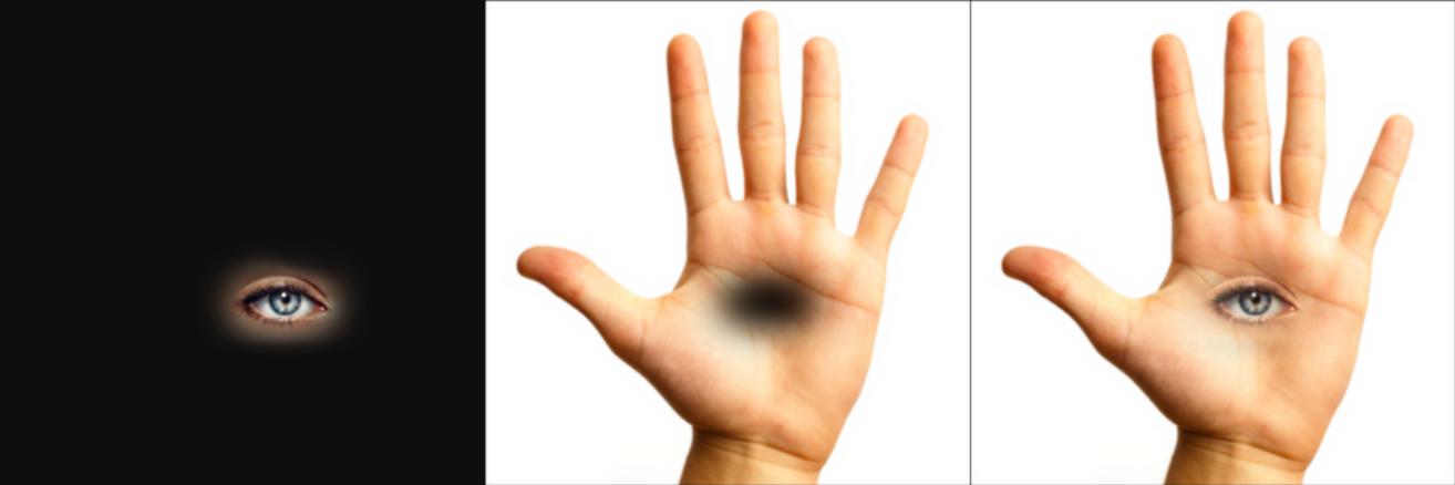
Part 2.4: Multiresolution Blending
Using the Gaussian and Laplacian stack implementations shown above, we produce results for two more images: another vertical spline image with a sunset and daytime landscape and an irregular mask blending an eye into a human hand. These results use the same technique of generating and summing a blended Laplacian stack as used to generate the oraple above.
Discussion
Takeaway: Gradients, Gaussians, and Laplacians are surprisingly effective tools for manipulating images (e.g. finding edges, blending images, sharpening, etc.) and the latest and greatest set of deep learning tools used for image processing may not necessarily be the most useful tool to pick first when attempting to extract some of the results shown above — frequencies are all you need! Additionally, I learned that perceptual quality is not necessarily correlated with the effectiveness of an algorithm, but largely due to careful input selection, masking, and parameter tuning (especially in the case of the Laplacian/Gaussian filter parameters for the blending and hybridization experiments).