This webpage contains two main sections, Part 1 and Part 2, with the corresponding subsections.
Image Credits are listed in the Jupyter Notebook in the corresponding calls from disk.
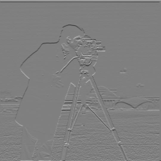
The visualizations are listed in the following order: partial derivative w.r.t x, partial derivative w.r.t y, gradient magnitude, and edge (threshold = 0.5)

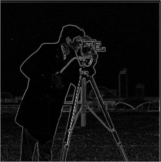
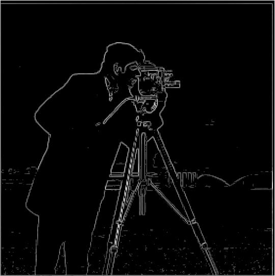
Here are the results when we filter then convolve (Gradient Magnitude and Edge (threshold = 0.20))
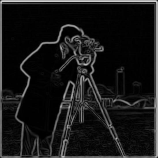
Comparison with Part 1.1: Edges are a lot more consistent, and we can see the full silhouette (edges) of the man and camera, rather than spotty lines. There's also relatively no noise within the image compared to the first technique.
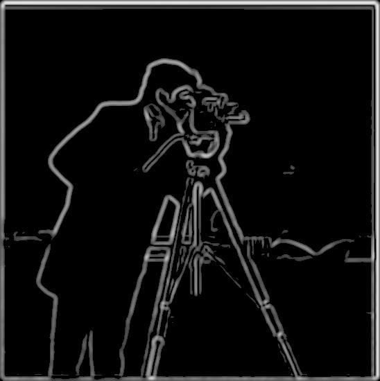
Here are the results when we convolve then filter (Gradient Magnitude and Edge (threshold = 0.20))
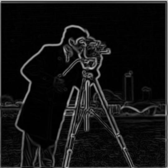
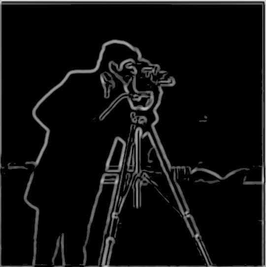
As shown, the order in which we convolve/filter is irrelevant and results in the same gradient magnitude and edge images.
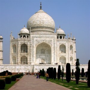
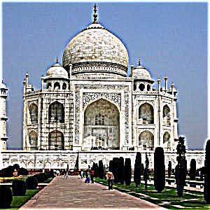
Here is a side by side comparison between the original and my sharpened version of taj.jpg. I used ksize=9, sigma=3, alpha=4 for my 2D Gaussian Kernel.
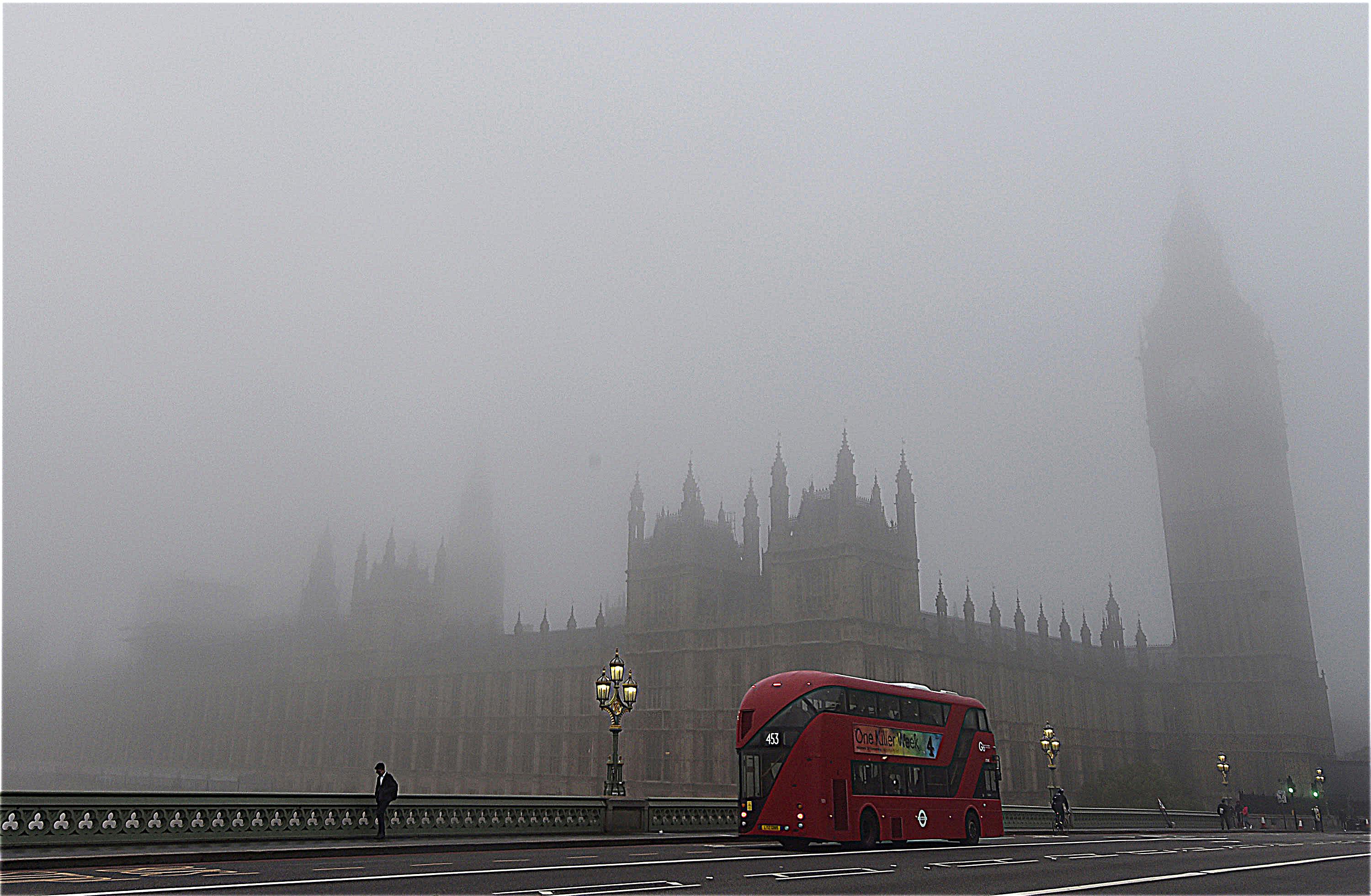
For my additional image, I wanted to see how sharpening increases the visibility of images. Thus, I chose a foggy image of the Palace of Westminster. Most structures seem more visible and outlined with sharpening, but those that are more occluded don't have sufficient information to bring out. We can also more easily read the analog clock on the Big Ben with the sharpened image! Here is a side by side comparison between the original and sharpened version. I used ksize=40, sigma=3, alpha=4 for the 2D Gaussian Kernel.

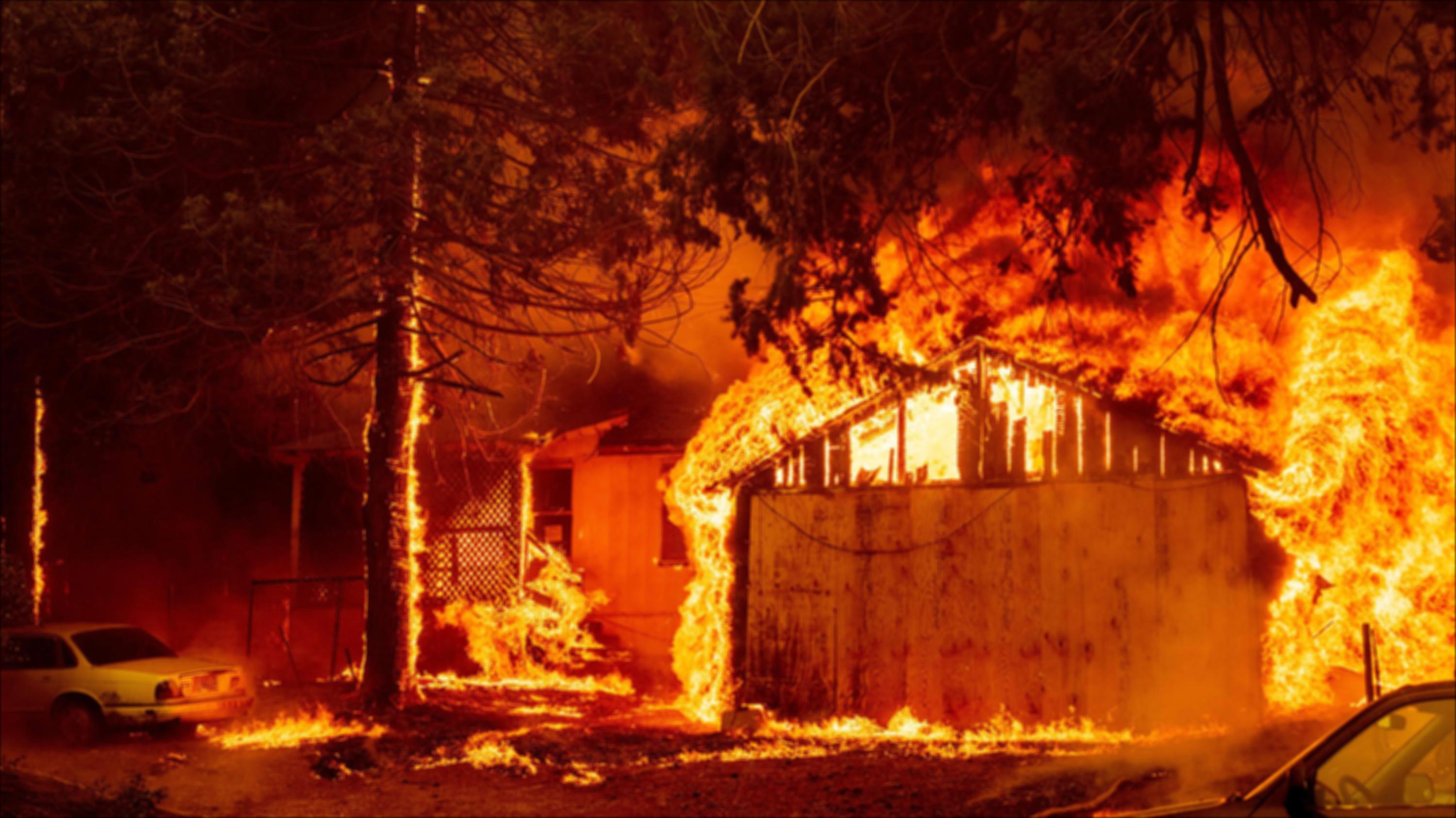
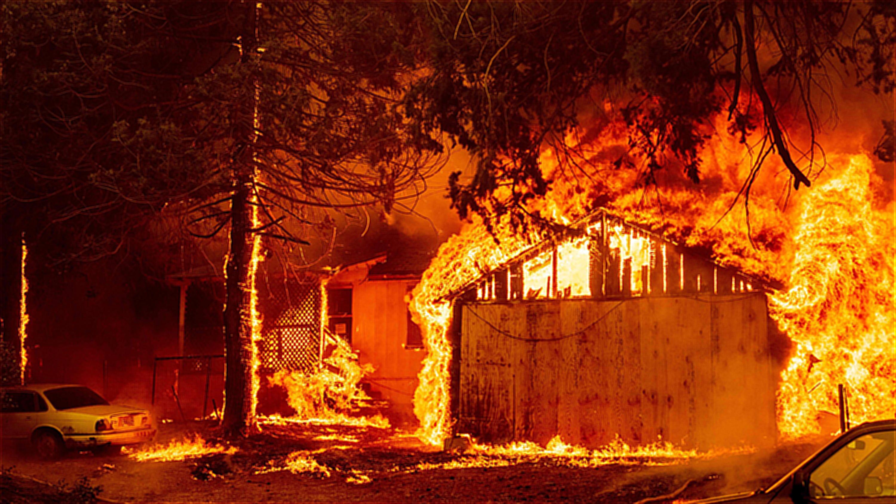
For my sharp-blur-sharp image, I chose this wildfire picture as it has a lot of very high frequencies (as fire would do in a photo). I wanted to test the limitations of sharpening when the image itself has an abundance of high frequencies. As you can see, with a larger filter, the sharpened image looks objectively better and smoother than the original image, which seems to have aliasing. Here is a side by side comparison between the original, blurred, and sharpened version. I used ksize=9, sigma=5 for the blurring 2D Gaussian Kernel and ksize=9, sigma=3, alpha=4 for the sharpening 2D Gaussian Kernel.

For reference, here is the finalized version of the sample hybrid image.
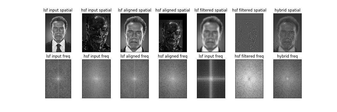
For my best hybrid image, I combined a terminator image (high SF) and a portrait of Arnold Schwarzenegger (low SF). I used the following parameters: sigma1 = 5, sigma2 = 5, ksize1 = 15, ksize2 = 9, alpha = 2. The visualization of the entire process in both spatial and frequency domain is shown below.
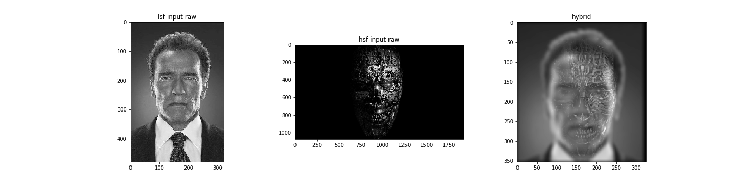
For my second hybrid image, I originally used a different terminator image (https://wallpaperaccess.com/terminator-skull), however I realized with the result that it looked more like a blend than hybrid, since the high frequencies in the terminator image only captured half of the face. The result looks pretty cool, but is not as hybrid as the previous or sample images. Fortunately, this can be counted as a blend or morph between the two images with some hybridization. I used sigma1 = 5, sigma2 = 5, ksize1 = 15, ksize2 = 15, alpha = 0.5 as my parameters. Here are the input raw images and final hybrid.
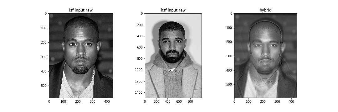
For my third hybrid image, I was inspired by the Donda > CLB debate and chose Kanye as my low SF image and Drake as my high SF image. I used sigma1=5, sigma2=5, ksize1=15, ksize2=15, alpha=0.75 for my parameters. Here are the input raw images and the final hybrid image.
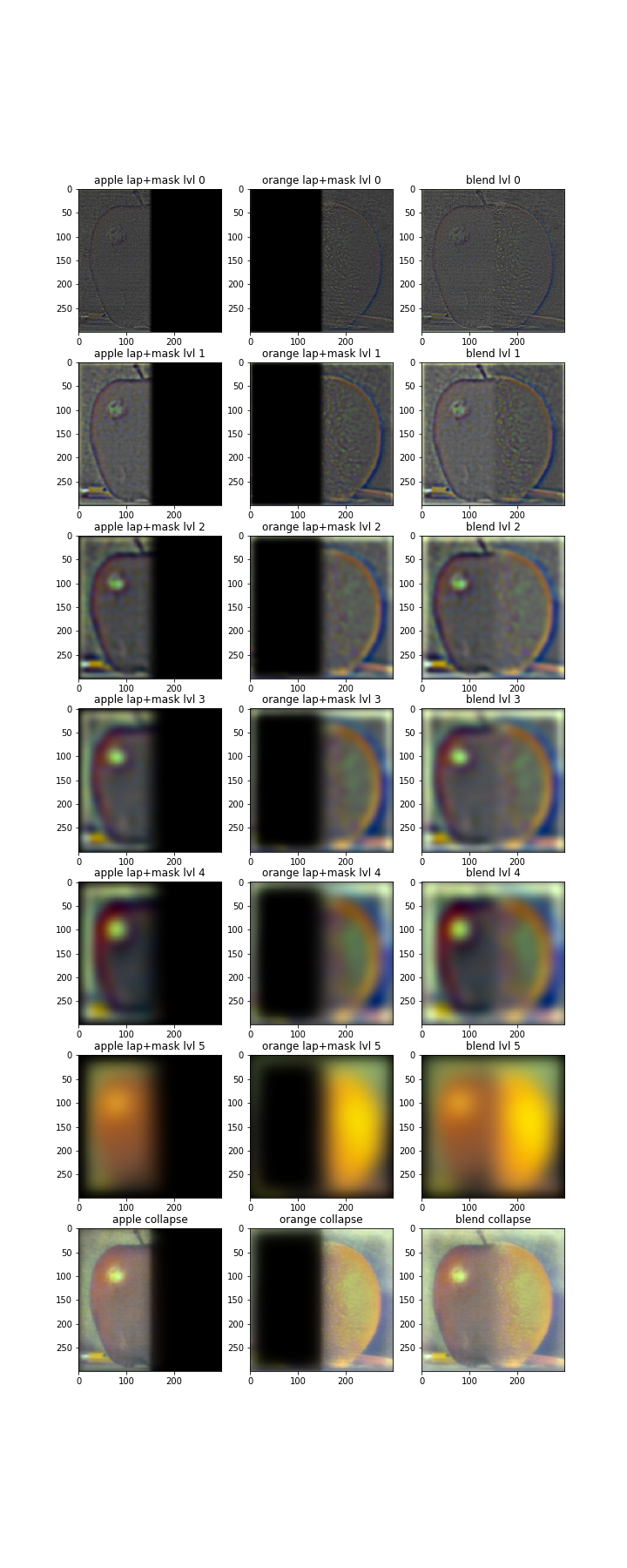
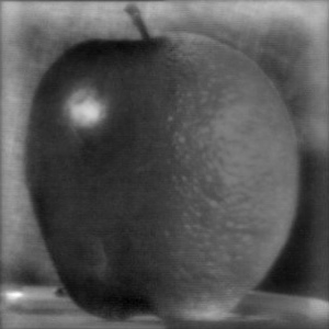
I used sigma=2, ksize=40 for my 2D Gaussian Kernel. Below are the oraple laplacian levels and the collapsed result in color alongside the grayscale final image for reference.
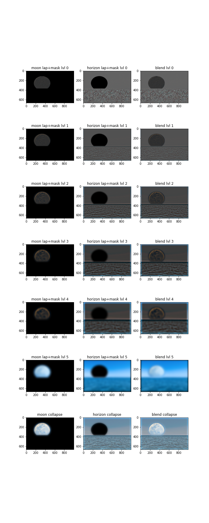
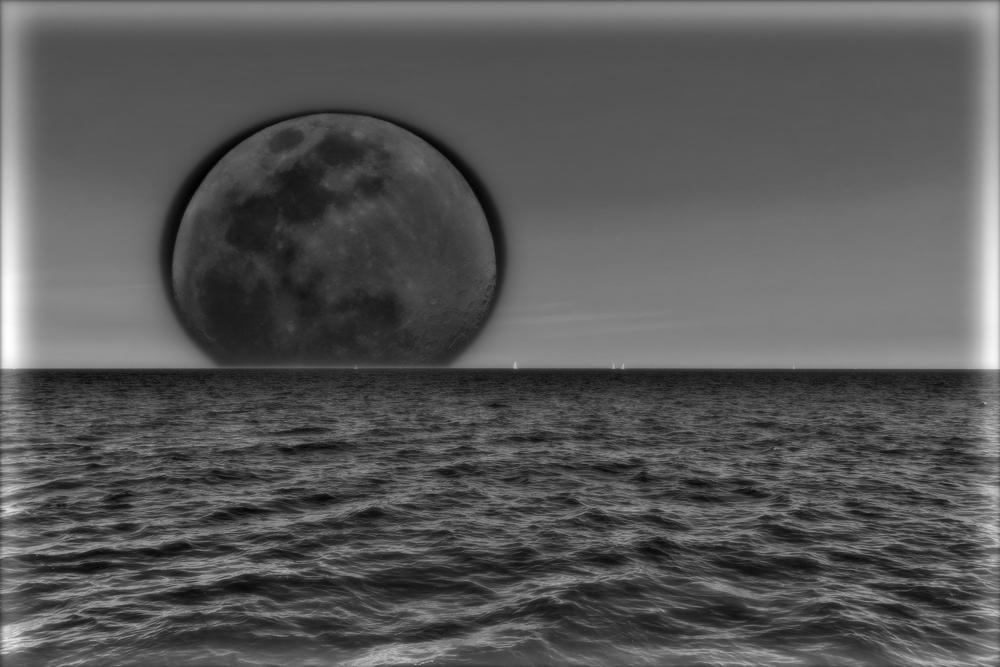
I used sigma=2, ksize=40 for my 2D Gaussian Kernel. I blended together the moon and the ocean horizon using a circular mask with a horizontal cutoff at the horizon line. Below are the corresponding laplacian levels and the collapsed result in color alongside the grayscale final image for reference.
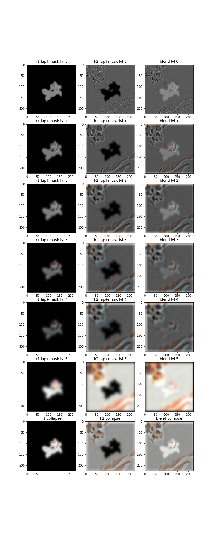
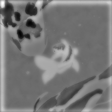
I used sigma=2, ksize=10 for my 2D Gaussian Kernel. I blended together two koi fish patterns by using a cookie cutter mask. Below are the corresponding laplacian levels and the collapsed result in color alongside the grayscale final image for reference.