Overview
In this project, I experimented with a variety of different filters to blur, sharpen, merge, and create hybrid
images. Almost all of the implemented filtering techniques can be derived from the Gaussian filter, which
serves as a low-pass filter over images. Building off of this, I played with high-pass filters to sharpen
images, manipulated frequencies of hybrid images to create different image intepretations at varying viewing
distances, and finally worked with Gaussian and Laplacian stacks to generate a smooth merging of images.
Part 1.1: Finite Difference Operator
 Partial Dx
 Partial Dy
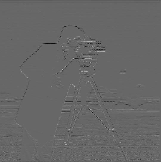
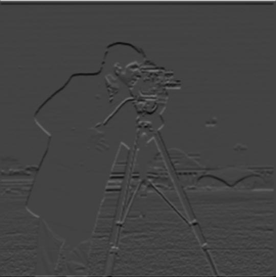
 Gradient Magnitude
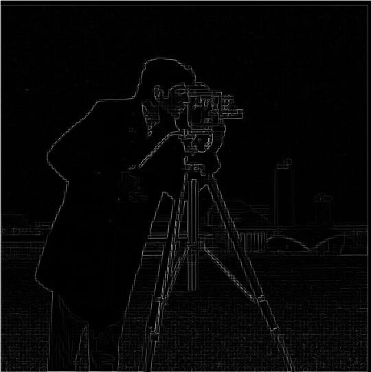
 Binarized Gradient MagnitudeThreshold = 0.28
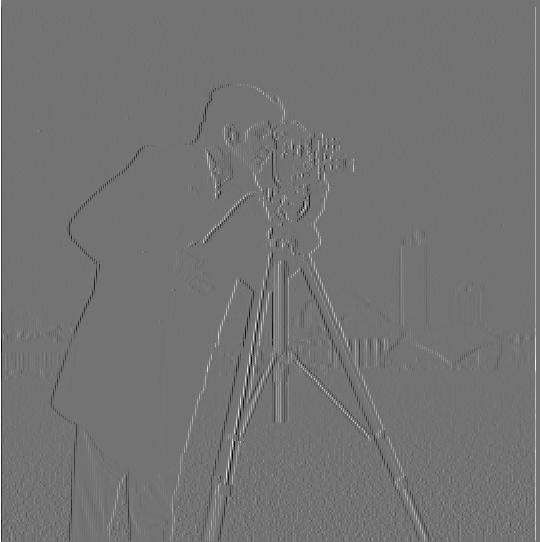
The gradient magnitude image is calculated by taking the square root of the sum of partial derivatives
squared. That is, grad_magnitude = sqrt(Dx^2 + Dy^2) where Dx is the partial derivative in X (calculated
by taking the convolution of the image with [1, -1]) and Dy is the partial derivative in Y (calculated by
taking the convolution of the image with [[1], [-1]]).
Part 1.2: Derivative of Gaussian Filter
 Blurred Partial Dx
 Blurred Partial Dy
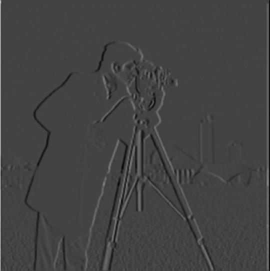
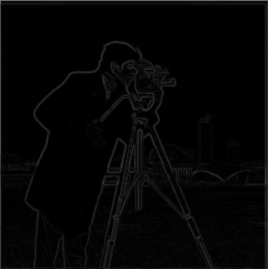 Blurred Gradient Magnitude
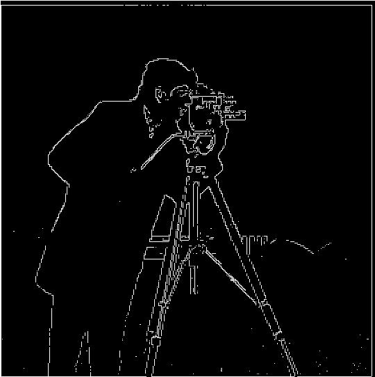
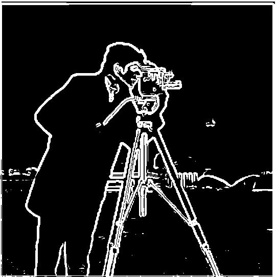 Blurred Binarized Gradient MagnitudeThreshold = 0.05
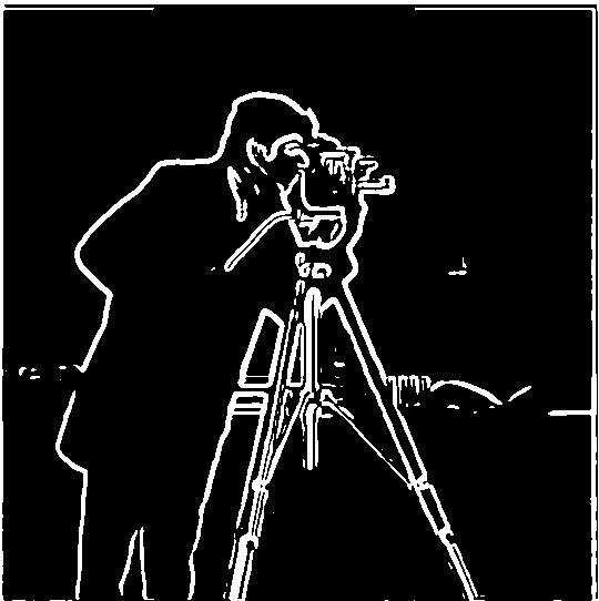
The above images show the same process as part 1.1 but with an additional convolution with a Gaussian
prior to creating the partial derivatives and gradient images. Applying the Gaussian convolution step has
the effect of adding a blur to the edges which makes the edges more prominent in the final binarized gradient
magnitude image. In the intermediate partial derivatives and gradient magnitude, we can similarly see that
the border edges are more pronounced and the images (at least for the partials) are noticeably darker.
One Convolution Verification
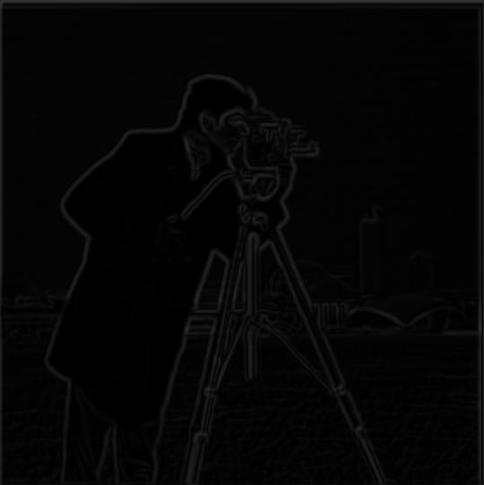 Blurred Gradient Magnitude
 Blurred Binarized Gradient MagnitudeThreshold = 0.05
 Blurred Binarized Gradient MagnitudeThreshold = 0.04
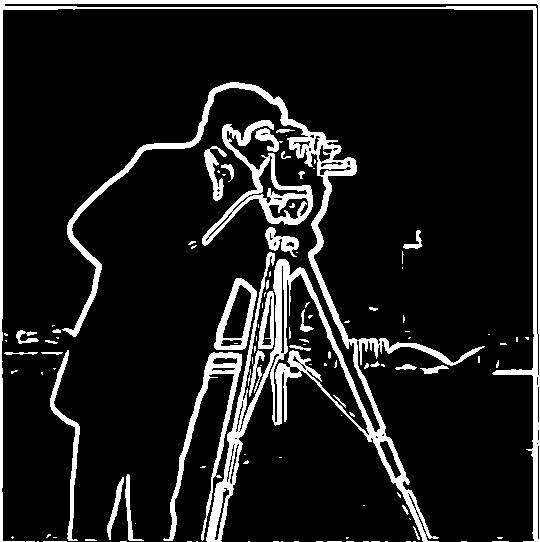
Applying the partial derivative convolutions onto the gaussian filter rather than directly on the image
produces roughly the same result. We can see that the gradient magnitude is significantly darker but the edges
that show up (while faint) look roughly the same as in the above blurred gradient magnitude. Due to being slightly
darker, I had to use a slightly lower threshold (of 0.04) in order to make the binarized image more similar to the one
achieved above.
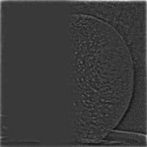
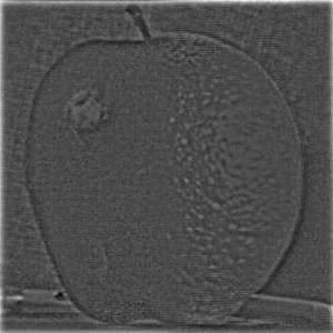
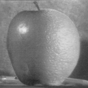
Part 2.1 Image "Sharpening"
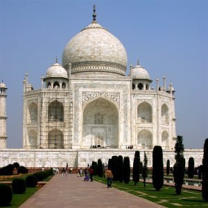 Original Image
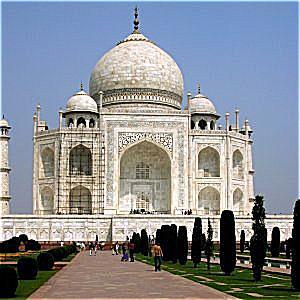 Sharpened imageAlpha multiplier = 1.5
 Original Monastery
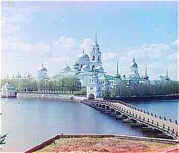 Sharpened MonasteryAlpha multiplier = 0.9
Sharpened images: The first pair is from the provided taj.jpg
image while the second is one that I chose from the Prokudin-Gorskii Photo Collection.
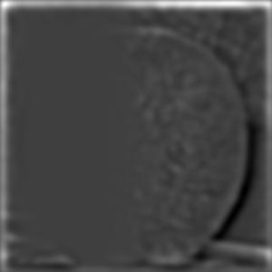
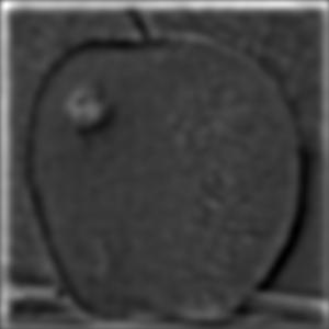
Blur then Sharpen Results
 Original Image
 Blurred image
 Re-sharpened imageAlpha multiplier = 8.5
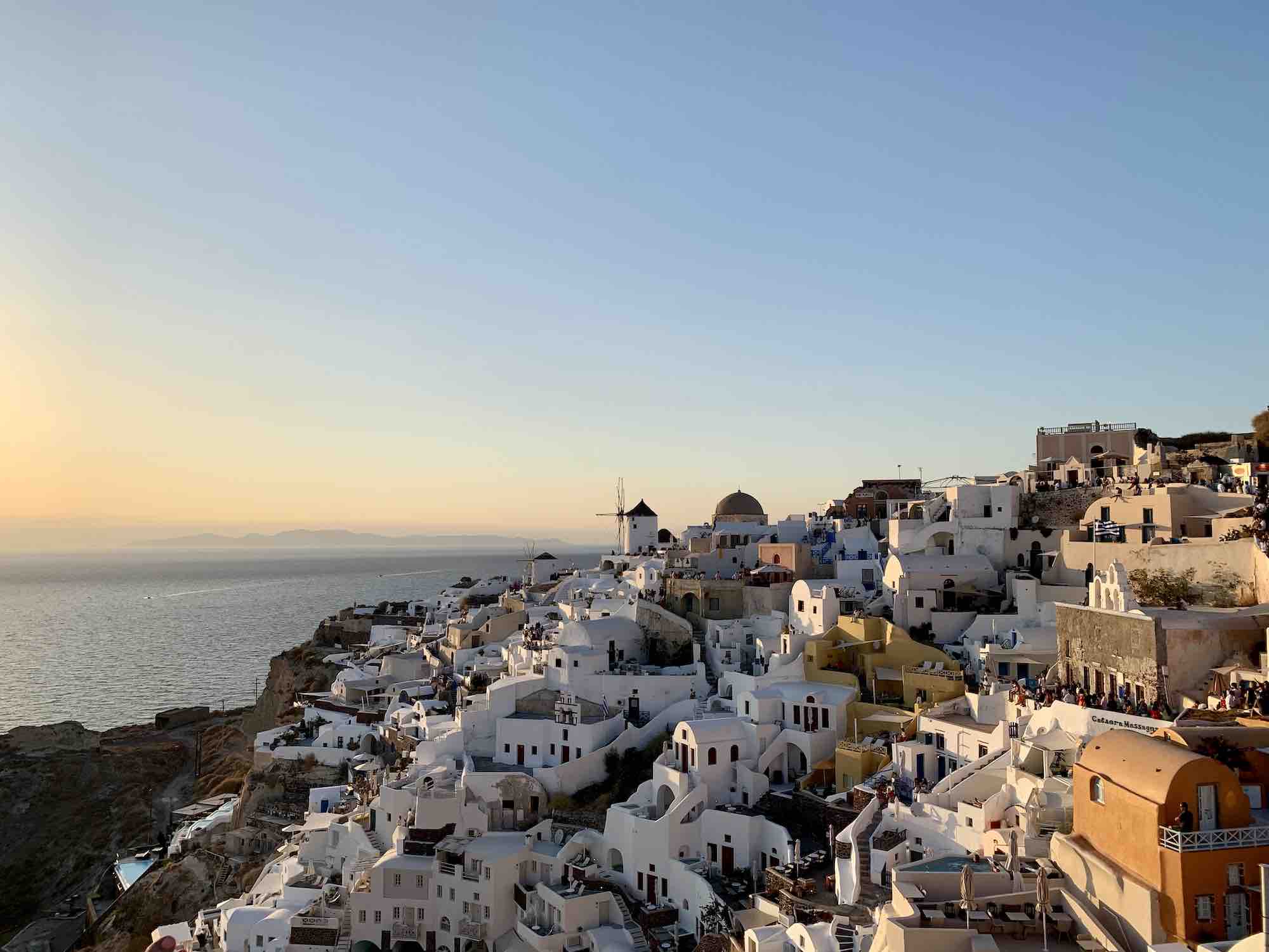
 Original Image
 Blurred image
 Re-sharpened imageAlpha multiplier = 8.5
Looking at the blurred and sharpened images, we can see that the re-sharpening does a very good
job of providing greater resolution of the image after blurring. However, in both of these photos,
it required a much higher high frequency multiplier in order to achieve almost the same resolution
result as the original image. (Blurring amount was done using size 10 kernels with sigma value of 3.)
One thing to notice is that the re-sharpening only really re-defines the edges, but the loss in color
contrast due to blurring is not retained (as can be seen in the sky of the top row images.) Meanwhile,
looking at the images in the bottom row, the original image has its focus on the foreground (the small weed)
and the background monument is a bit blurred to begin with. After blurring and re-sharpening, the re-sharpened
image seems to attempt to define some of the edges in the background, creating more severe cracks and edges
in the monument that weren't as well-defined in the original. Additionally, the weed in the foreground is not as
precisely outlined as in the original.
Part 2.2: Hybrid Images
Provided Derek/Nutmeg hybrid
 Nutmeg Image
 Hybrid image (close)
 Hybrid image (far)
 Derek Image
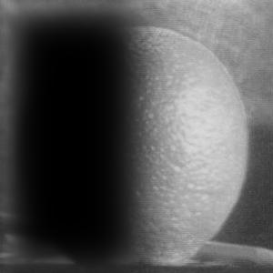
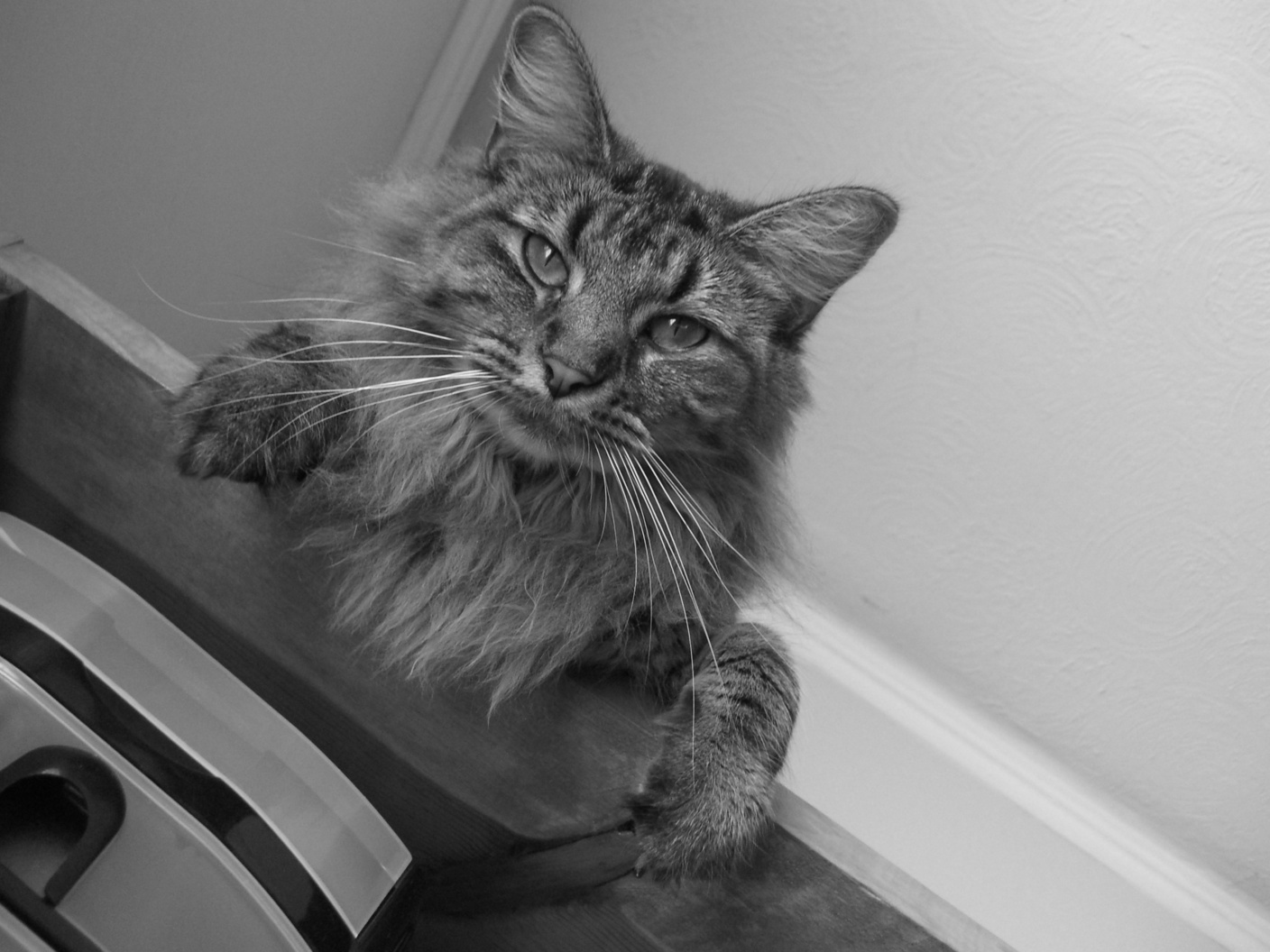
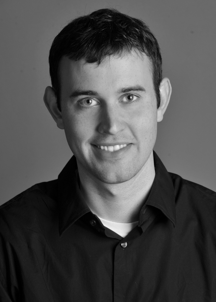
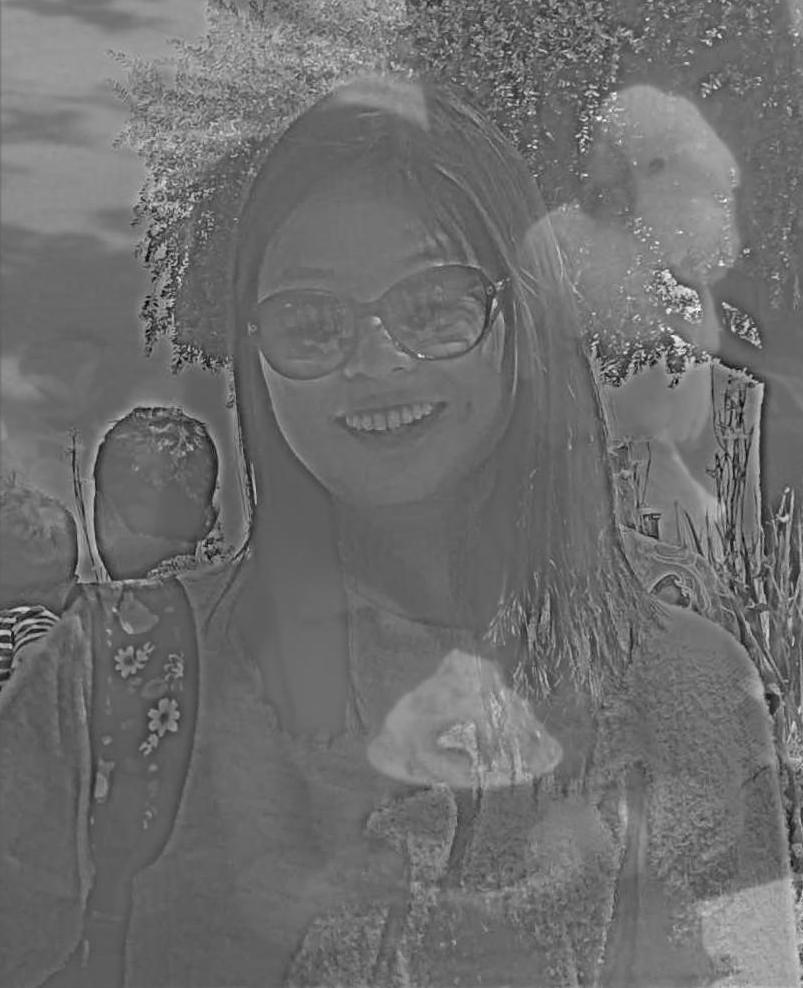
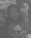
Me and a bird hybrid
 Me and a bird (at 19)
 Hybrid image (close)
 Hybrid image (far)
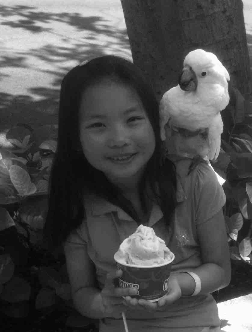 Me and a bird (at 11)
I found that putting a hybrid of me at 19 with a bird using high frequency and me at 11
with a (different but similar looking) bird at low frequency worked pretty well. This is because the more recent
photo of me has a lot higher resolution which worked well in extracting out the high frequencies
for close distance viewing while the photo of me at 11 was taken a long time ago with a worse iphone camera
so the low frequencies worked well as a background that is visible in far distances. As a failure example, I also
tried doing it the opposite way (using the more recent photo as the low frequency and the photo of me
at age 11 with high frequency) and this did not work well at all. Results are shown below. I believe this is
due to the fact that the photo of me at 11 did not have as much high frequency in terms of the facial
features and hair so it's very hard to distinguish since not a lot of high frequency signal was able to get through
the high frequency filter and overlay on top of the more recent photo of my face. As a result, we get a very
odd-looking baby face filter that is partially visible and an extremely pronounced bird outline in both close and far
viewing distances. (I had to crank up the high frequency visibility in order to get the baby-version of myself to
even show up which made the white bird and ice cream very pronounced.)
Me and a bird hybrid failure
Me and a bird (at 11)
 Hybrid image (close)
 Hybrid image (far)
Me and a bird (at 19)
Some hybrid images that don't involve me (A dog and a llama)
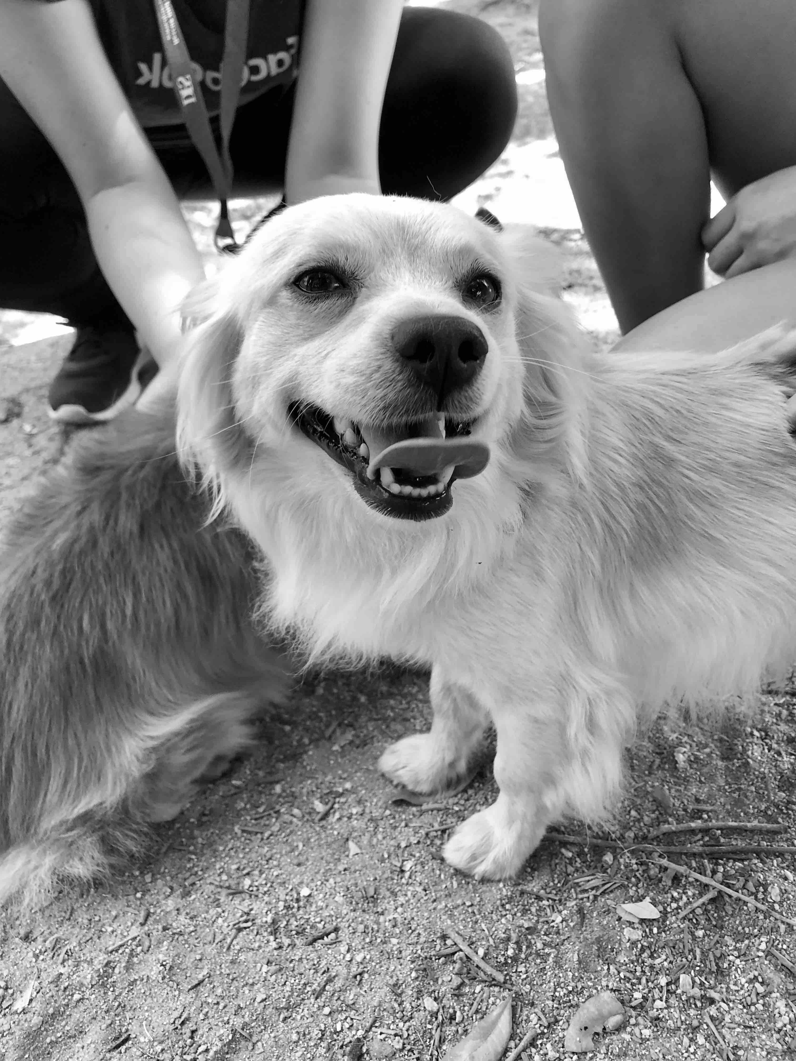 Dog
Dog
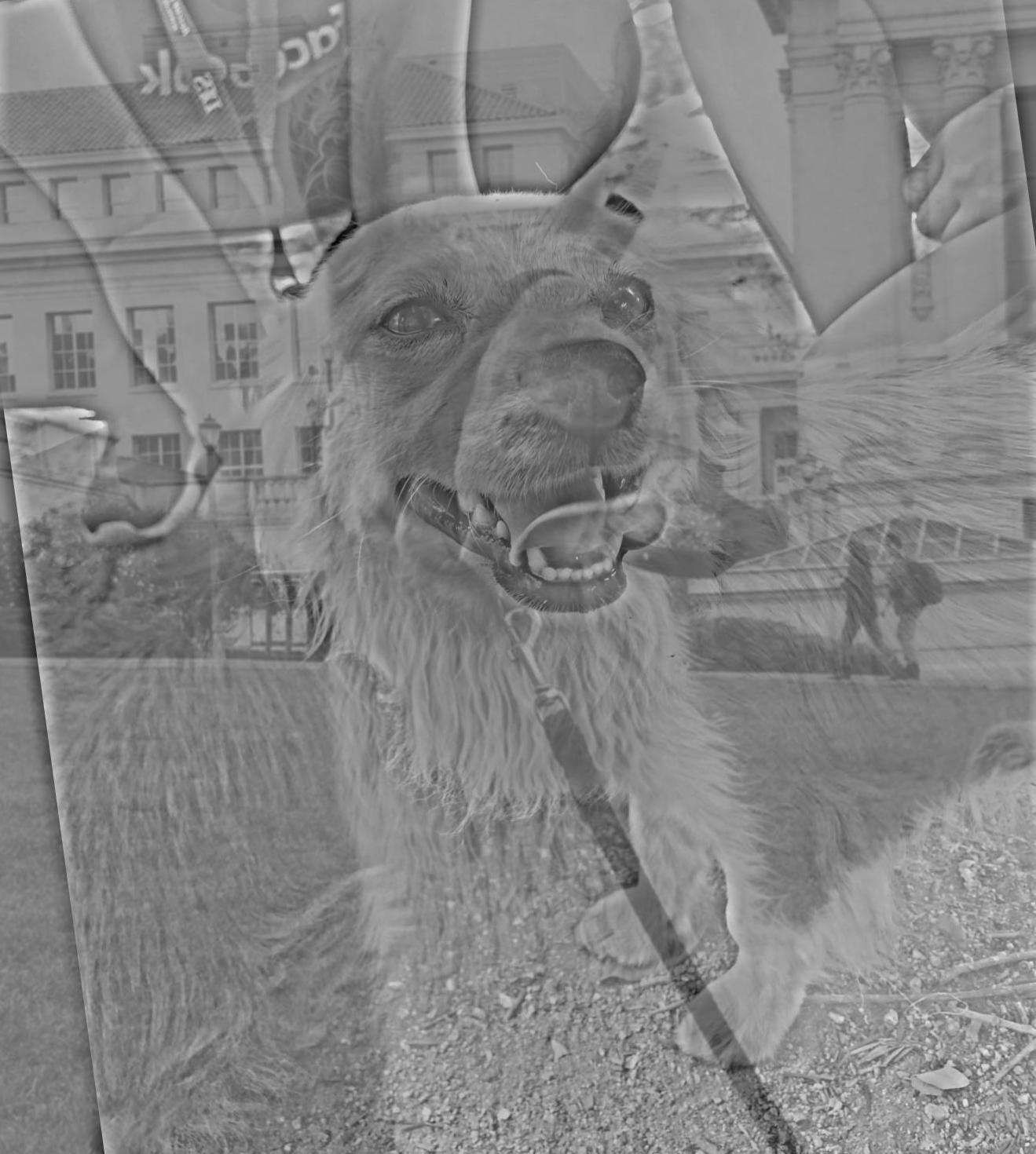 Hybrid image (close)
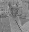 Hybrid image (far)
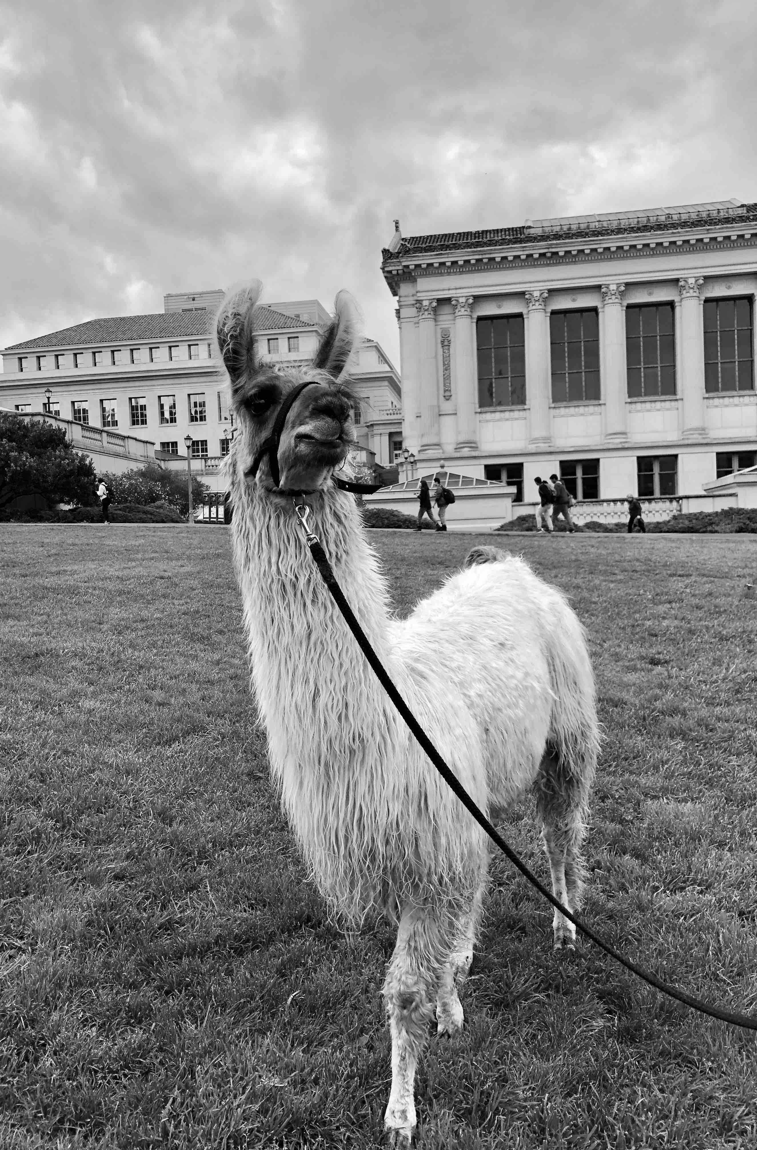 Llama
Llama
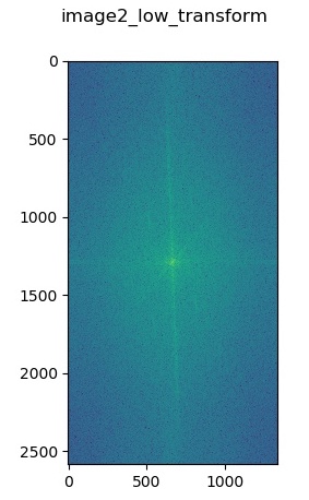
These are two animal photos in my camera roll. I found that creating a hybrid out of these turned
out pretty well since both animals have a similar angle of head tilt and the dog has a tongue sticking
out which gives it a lot of high frequency data that is very clearly pronounced in the closeup while the
llama's closed and slightly uptilted mouth is visible in the far distance image. The frequency analysis
for each of these images is as follows:
 Log Fourier transform of input dog image
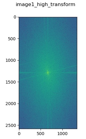
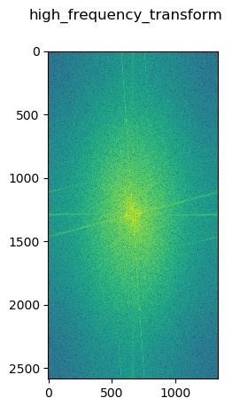 Log Fourier transform of high frequency filtered dog image
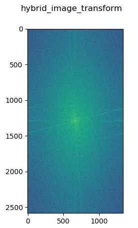 Log Fourier transform of hybrid image
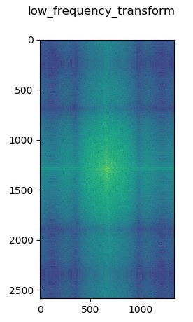 Log Fourier transform of low frequency filtered llama image
 Log Fourier transform of input llama image
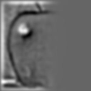
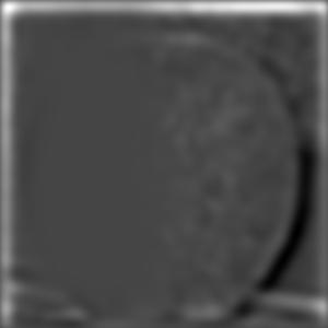
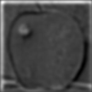
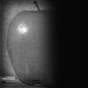
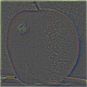
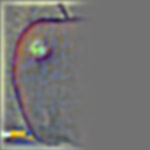
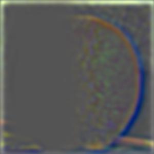
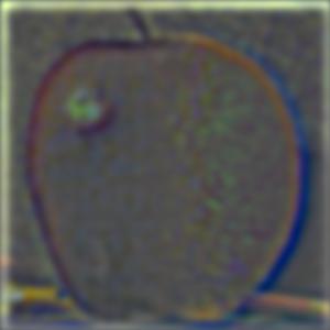
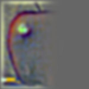
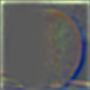
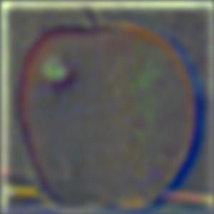
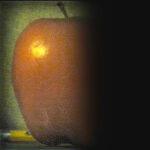
Part 2.3: Gaussian and Laplacian Stacks
Laplacian Pyramid
(Regular Black/White)
Laplacian Pyramid
(Bells & Whistles Color)
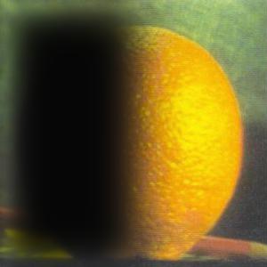
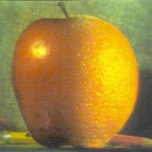
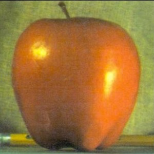
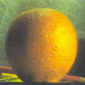
Above are two Laplacian pyramids for left, right, and combined laplacians run on the
provided apple and orange inputs.
Part 2.4: Multiresolution Blending
Normal Mask
Irregular Mask
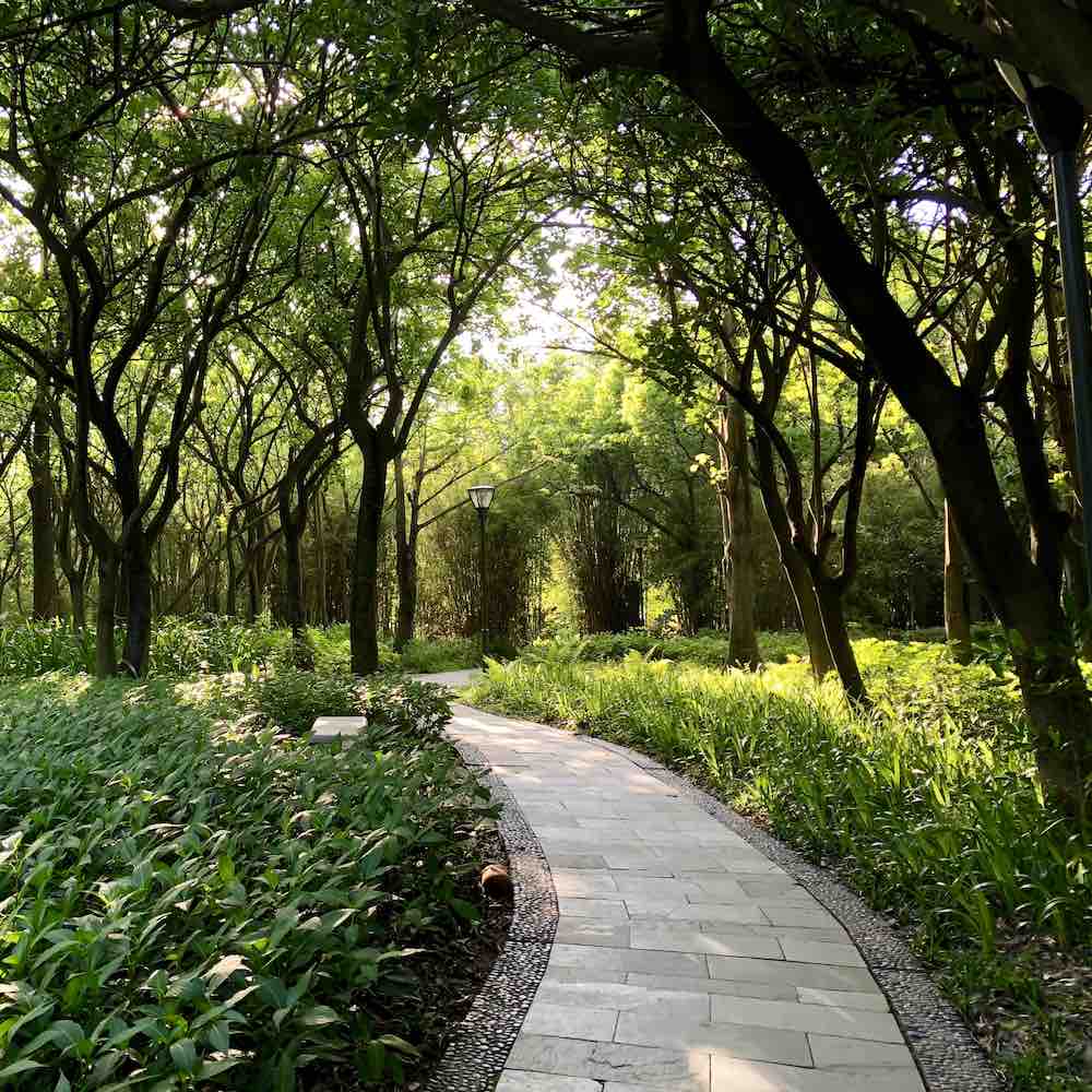 Forest trail
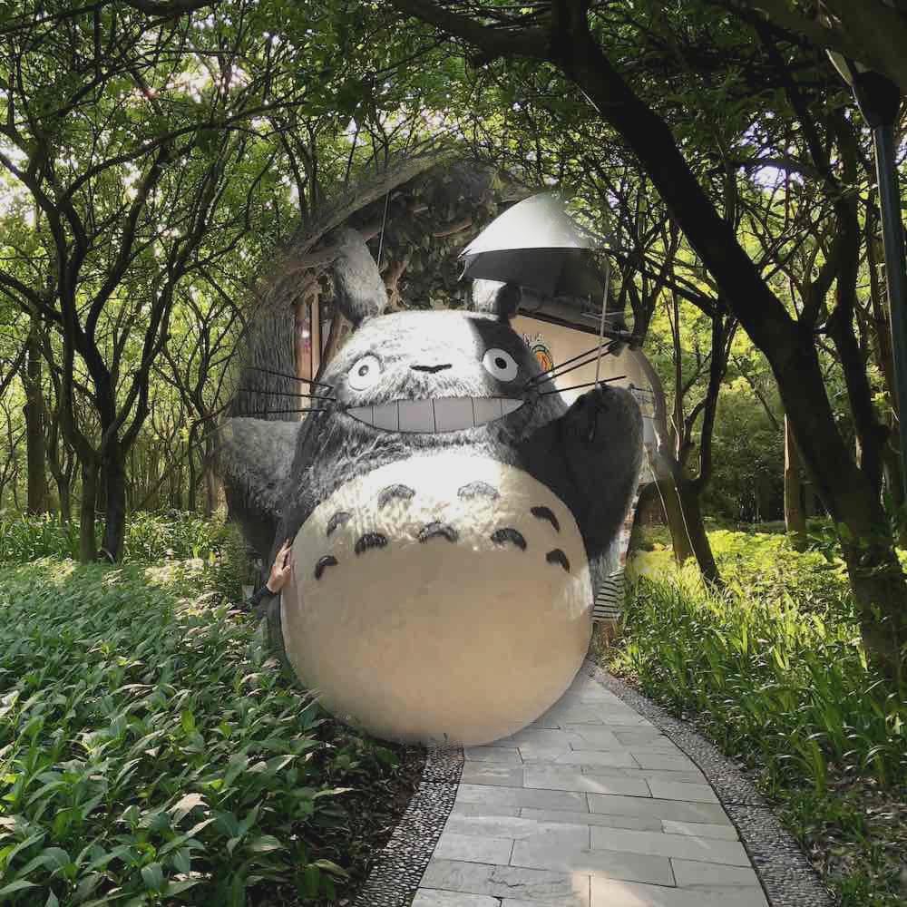 Blended image
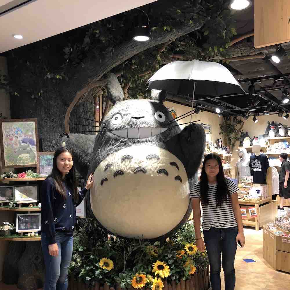 Totorro
Here is a multiresolution blending of totorro in a park trail. I created an irregular
mask that is an oval shape which surrounds the main part of the totorro structure and placed it
inside an image I took of a park forest trail.
Conclusion
The coolest and most interesting thing I learned from this project was probably creating the unsharp
mask filter for sharpening images. When I take pictures, the most often complaint is lack of resolution so
I thought it was super cool to learn that sharpening an image is actually not that difficult--and in fact,
can be achieved by creating a blured version of the image (which was quite contrary to what one might
imagine!). The unsharp mask filter also provides a very clear and clean way of sharpening an image with one
convolution so I found it really useful, simple, and applicable for many cases.
One of the most important things I learned in this project is how convolutions work in the manipulation of images
and image frequencies. All of the above methods rely foundationally on convolutions with a Gaussian and it was really interesting
to learn why Gaussians were the popular filter choice (due to its shape and fourier transform) and work hands-on with
different applications of Gaussians and see the wide myriad of image manipulations that can be achieved just from
applying a convolution in a different order or method.