Dx
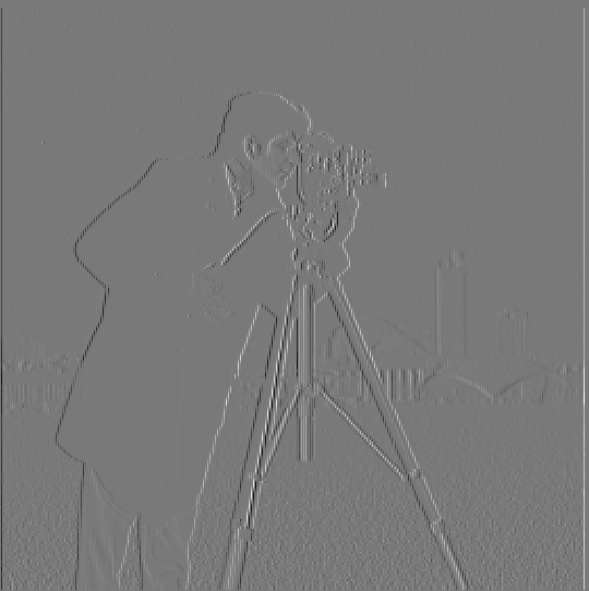
Dx = [[1, -1]]
Dy
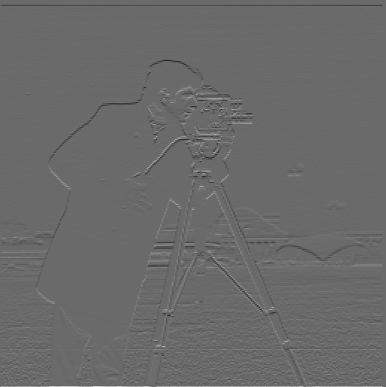
Dy = [[1], [-1]]
gradient magnitude
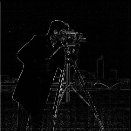
gradient magnitude = sqrt((im/dx)**2 + (im/dy)**2)
threshold
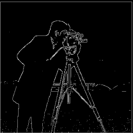
threshold = 0.23
We first compute the partial derivatives of the cameraman image by convolving the image with the Dx and Dy arrays. Once we have the Dx/Dy convolved images, we can use the gradient magnitude to detect edges in our image. Gradient magnitude is calculated by squaring both of the images, adding them together, and then taking the square root of the resulting image. I made use of the numpy.hypot() and passed in the two Dx/Dy images as arguments and the resulting image was the gradient magnitude. After retrieving the gradient magnitude, I used a threshold to suppress the noise while keeping true edges. I reached my threshold through qualitative assessment of various threshold values.
Dx

Dx = [[1, -1]]
Dy

Dy = [[1], [-1]]
gradient magnitude

gradient magnitude = sqrt((im/dx)**2 + (im/dy)**2)
threshold

threshold = 0.23
Using the Gaussian filter blurs the image, with the right sigm and kernel size, our Gausian filter can allow us blur the edges so they aren't so sharp and achieve the true edges more smoothly/clearly opposed to the harsh/noisy image from the previous part. Here are the results of the above but using a Gaussian filter on the image beforehand.
Dx
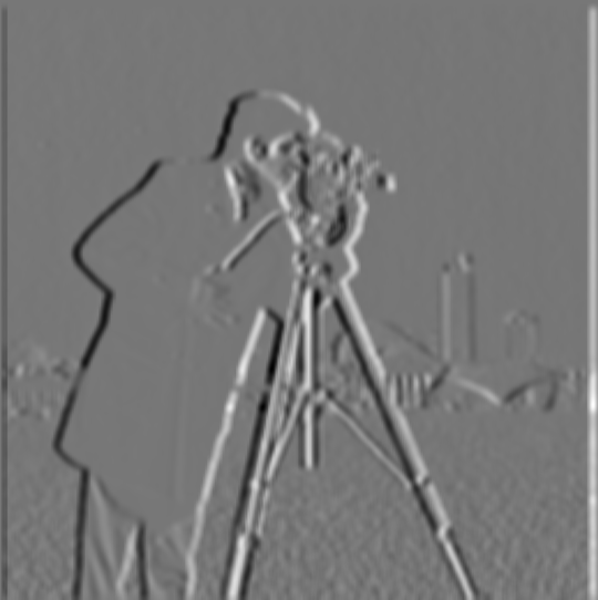
Dx = [[1, -1]]
Dy
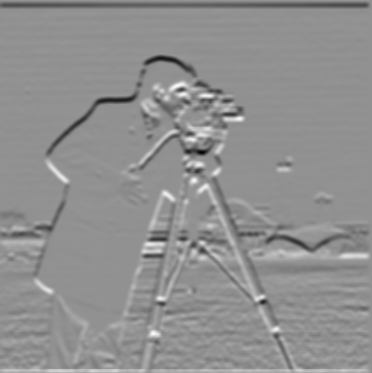
Dy = [[1], [-1]]
gradient magnitude
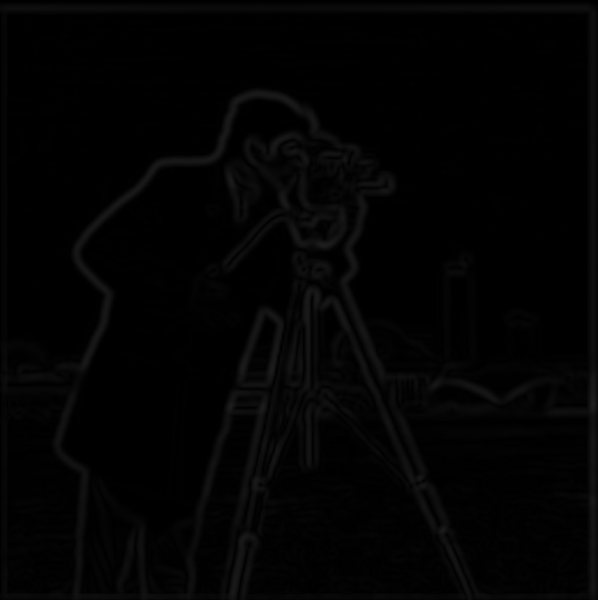
gradient magnitude = sqrt((im/dx)**2 + (im/dy)**2)
threshold
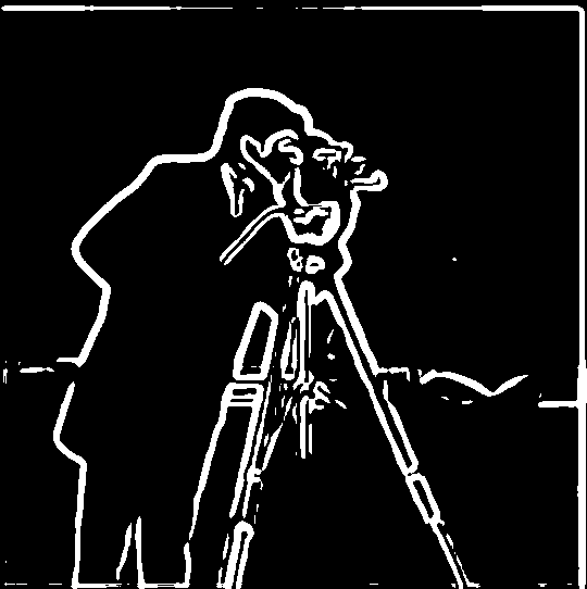
threshold = 0.04
Using the Derivative of Gaussian (DoG) filter allows us to achieve the same results by applying associativity with convolutions. Here are the results of this process. Note: I used the 'same' mode when convolving so there are some minor discrepancies but this can be chalked up to numerical precision.
Dx
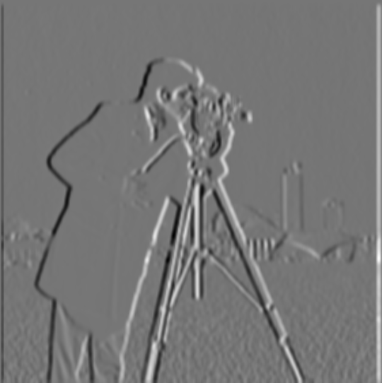
Dx = [[1, -1]]
Dy
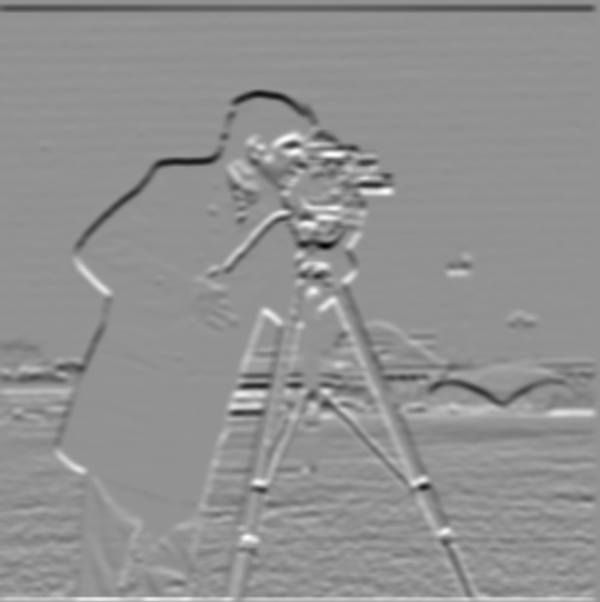
Dy = [[1], [-1]]
gradient magnitude

gradient magnitude = sqrt((im/dx)**2 + (im/dy)**2)
threshold
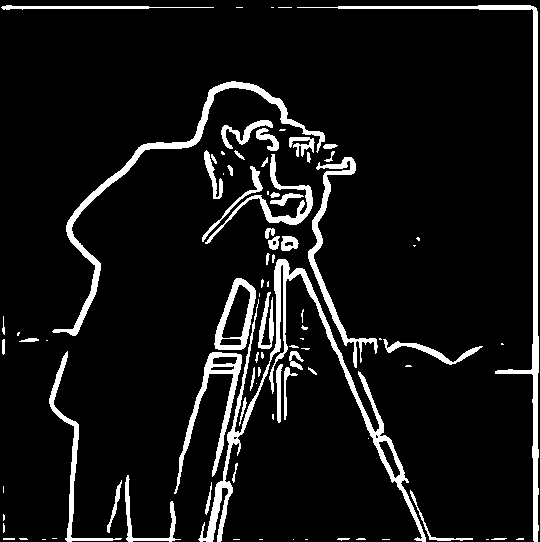
threshold = 0.03
In this part, we applied the unsharp mask filter and used some smart math to only have to do one convolution. Note: the sharpened image is visibly darker and grayer. I attempted to make this better by clipping the values to be bounded between 0 - 255 but sharpening still leaves some dark traces behind (in order to see the edges better).
Original Image
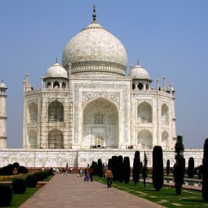
alpha = 0
Sharpened Image

alpha = 1
Original Image
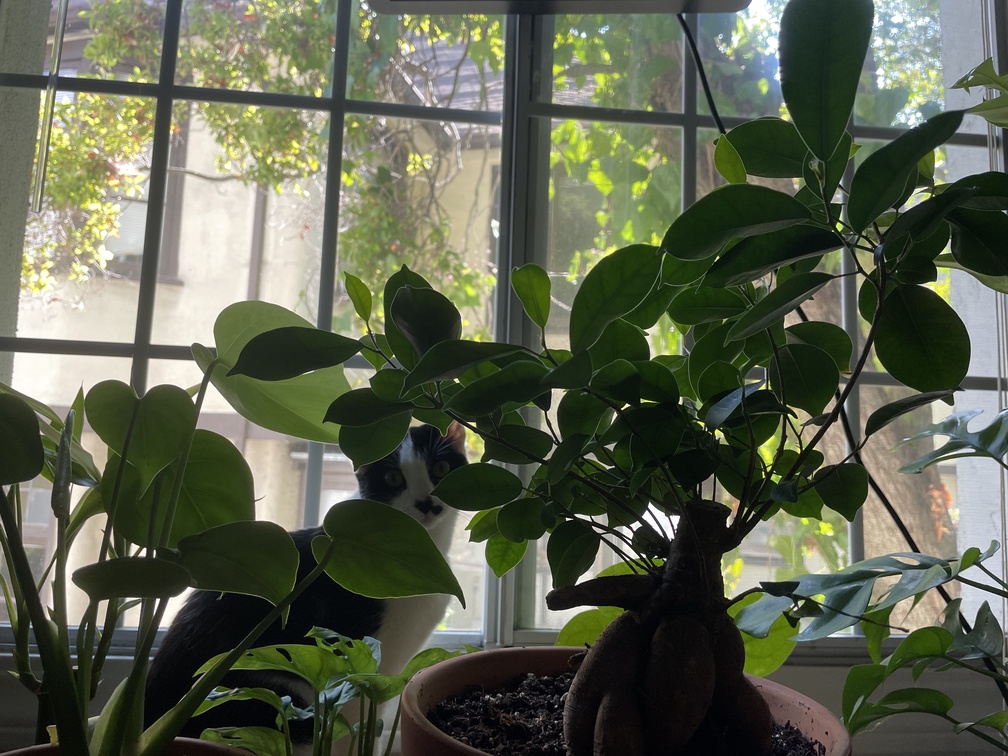
alpha = 0
Sharpened Image
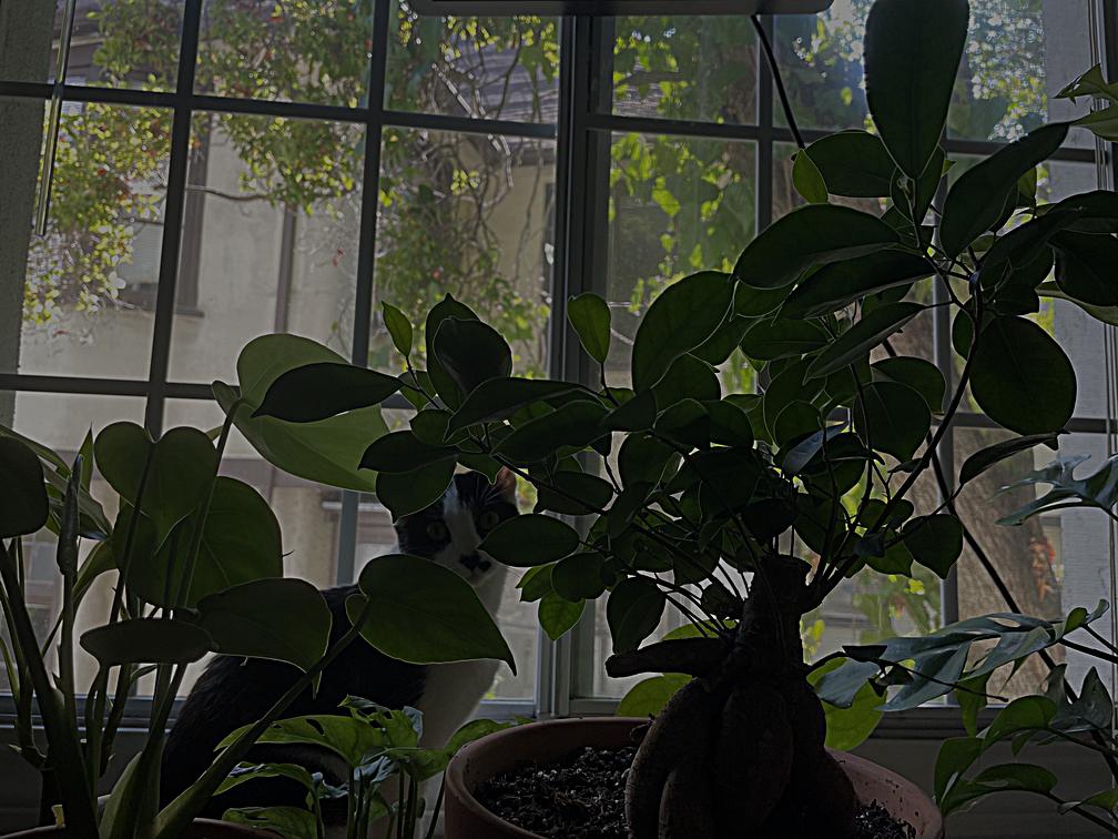
alpha = 1
We can also examine how sharpening looks on an already sharp image. Below, I used the sharpened taj photo from above and applied the unsharp mask filter on it again after blurring. Look at the results below.
Original Image

alpha = 0
Sharpened Image

alpha = 1
Sharpened -> Blurred -> Sharpened Image
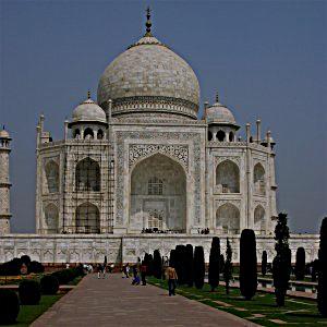
alpha = 1
As you can see, there isn't too great of a difference between the 2nd and 3rd image. This may be due to choice of sigma, kernel size, or alpha but all I can tell is the 3rd image is slightly darker. If the differences were more obvious, I would hypothesize that the far right image would become more accentuated and the lines would get thicker/darker and generally be more obvious.
This part was really cool. We take the low frequencies of one image, the high frequencies of another, and combine the two so that we see different images at different frequencies. We use a low pass filter to get the low frequencies, high pass filter to get the high frequencies and add them together (can average them as well). Another important part in this process is to choose images that are similar enough that their stacking goes well together and then you must align them so features overlap (necessary to make it realistic as possible). For the high pass filter, I used a kernel with size 7x7 and sigma = 6. For the low pass filter, I used a kernel with size 19x19 and sigma = 6. These cutoff frequencies were chosen qualitatively and hard to choose. Here are my favorite results:
Input Image #1
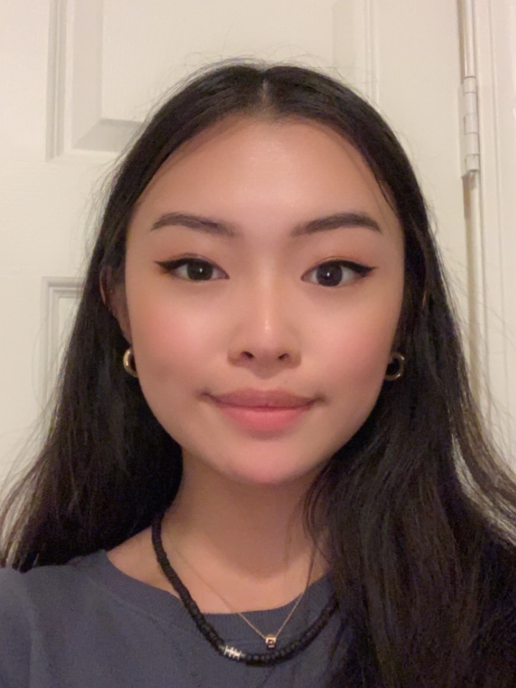
My girlfriend, Alex
Input Image #2
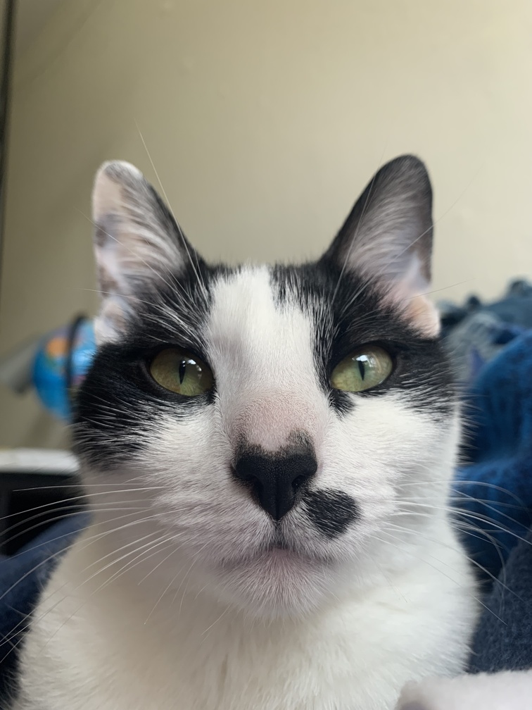
My cat, Gemma
Hybrid Image
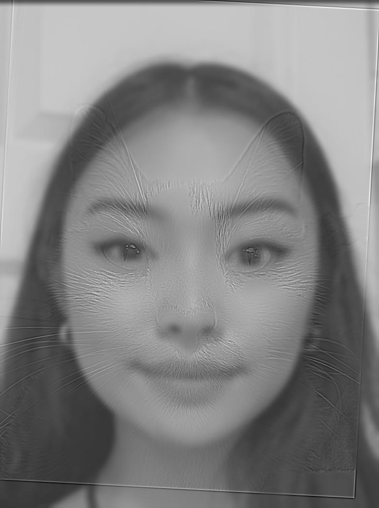
Gemex / Alemma
This one probably turned out the worst of the three. First the images don't have too many overlapping features. Also, the picture of Gemma was hard to retrieve the high frequencies without messing up the high pass for the next two hybrid images (I used the same kernel for all hybrid images). Still a cute hybrid though.
Input Image #1
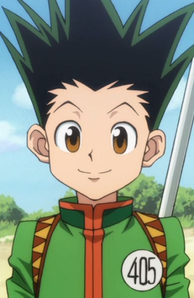
Gon
Input Image #2
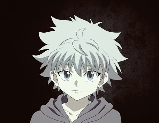
Killua
Hybrid Image
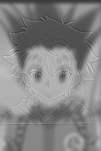
Gillua / Kon
This was the first hybrid image I tried and I really like it! The features overlap really well and Killua's brighter/white hair and skin works really well as the high frequency component of the image. For copyright purposes, I got Gon's image from here and Killua's image from here.
Input Image #1
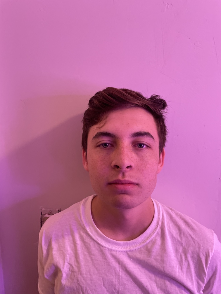
My friend, Jack
Filtered Input Image #1
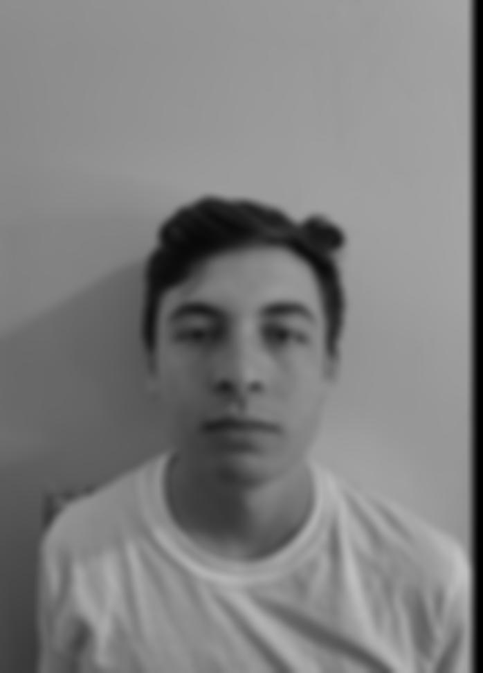
My friend, Jack but low
Input Image #2
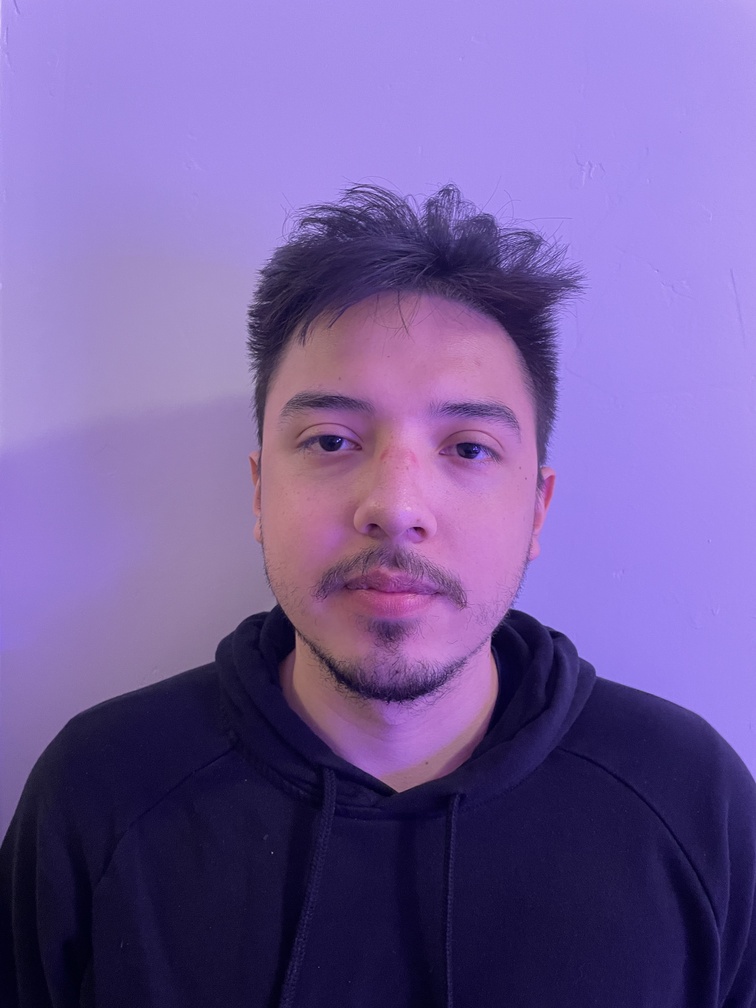
My friend, Jack
Filtered Input Image #2
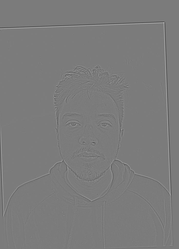
My friend, Steve but high
Hybrid Image

Jeve / Stack
This one is my favorite of the three. The hybrid image turned out REALLY well (might not look that good on the site since the image is small but that means it's working because you can only see the low frequency image, Jack). This one worked out so well because I took their images myself and had them stand at the same distance with the same facial expression. Their facial features overlap for a scary good hybrid image. Below is the FFT versions of each image above.
FFT Input Image #1
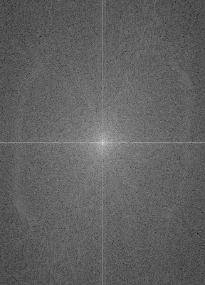
My friend, Jack but FFT
FFT Filtered Input Image #1
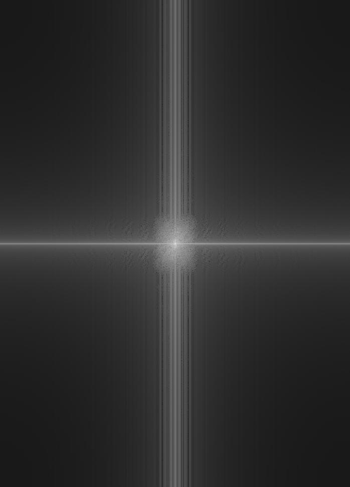
My friend, Jack but low and FFT
FFT Input Image #2
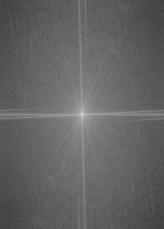
My friend, Steve but FFT
FFT Filtered Input Image #2
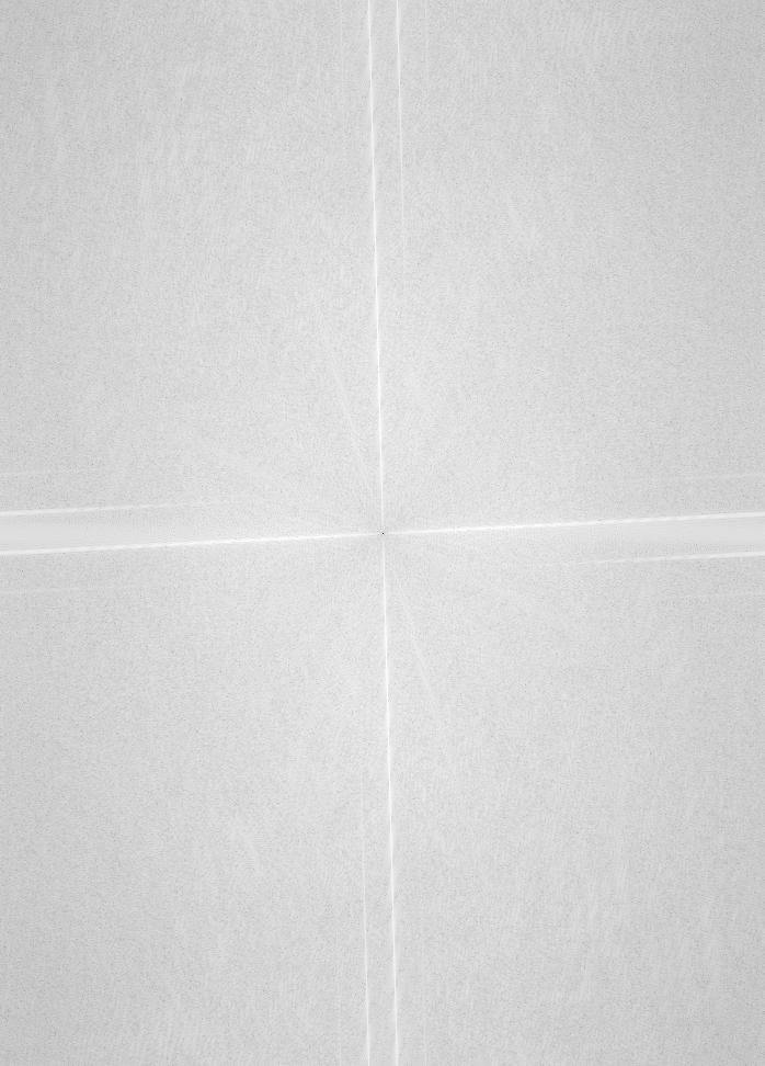
My friend, Steve but high and FFT
FFT Hybrid Image
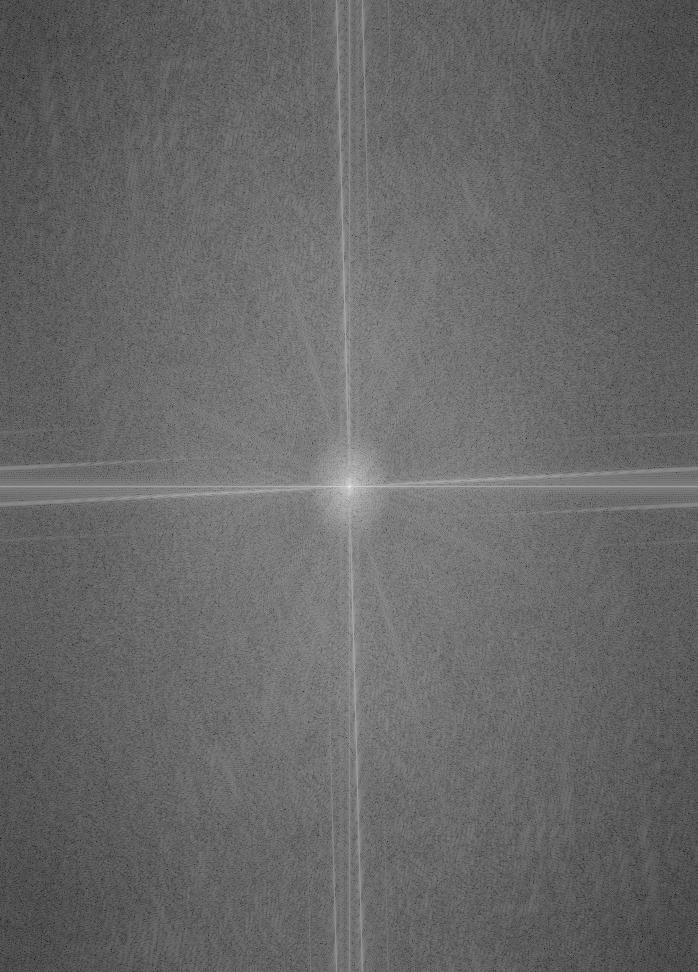
Jeve / Stack but FFT
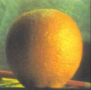
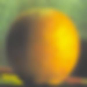
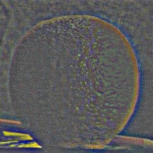
In this part, we create the Gaussian and Laplacian stacks to develop a multiresolution blending and discover the truth behind the oraple. I used a Gaussian Kernel with size 25x25 and sigma = 8. Below are the Laplacian and Gaussian Stacks of the orange and apple example images. Note: the last layer of the Laplacian stacks are the same as the last layer of the Gaussian stacks so that we can add up the Laplacian stack to retrieve the original image.
Gaussian Stack - Apple
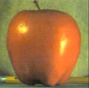
Depth 0
Gaussian Stack - Apple

Depth 1
Gaussian Stack - Apple

Depth 2
Gaussian Stack - Apple

Depth 3
Gaussian Stack - Apple
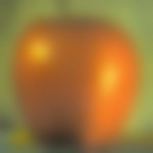
Depth 4
Gaussian Stack - Orange
Depth 0
Gaussian Stack - Orange
Depth 1
Gaussian Stack - Orange

Depth 2
Gaussian Stack - Orange
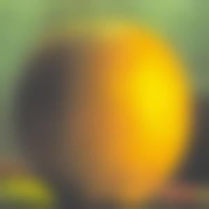
Depth 3
Gaussian Stack - Orange

Depth 4
Laplacian Stack - Orange
Depth 1
Laplacian Stack - Orange
Depth 2
Laplacian Stack - Orange
Depth 3
Laplacian Stack - Orange
Depth 4
Laplacian Stack - Orange

Depth 5
Laplacian Stack - Apple
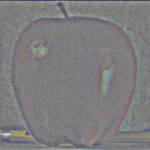
Depth 1
Laplacian Stack - Apple
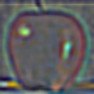
Depth 2
Laplacian Stack - Apple
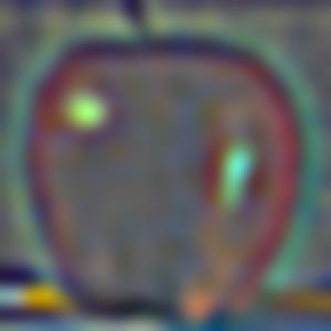
Depth 3
Laplacian Stack - Apple
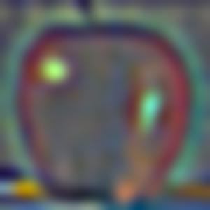
Depth 4
Laplacian Stack - Apple

Depth 5
Here, we took our Laplacian stacks from above and blend two images together using a mask (that has a gaussian filter applied to it as well). The resulting image should be an image that blends together smoothly to produce one, single image.
Original Apple

left
Original Orange

right
Mask

Vertical Mask
Oraple
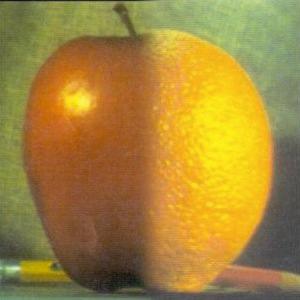
blended
Here is one set of extra blended images I put together, using the previous images of Jack and Steve. The black and white looks better so I included that too
Jack

left
Steve

right
Jeve / Stack BW
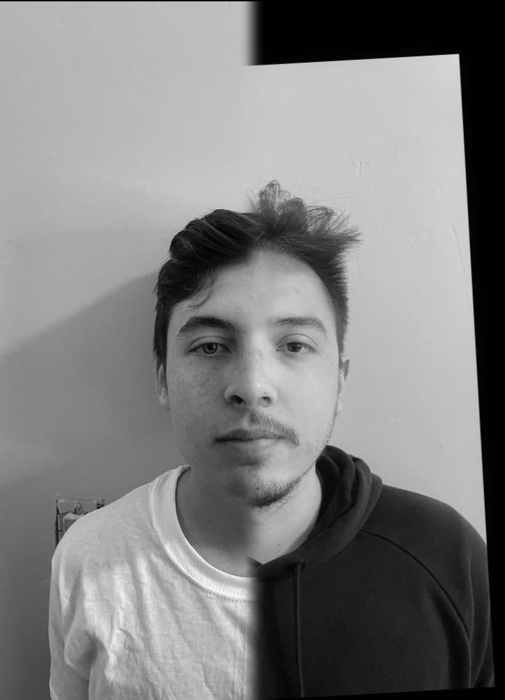
blended (black & white)
Jeve / Stack
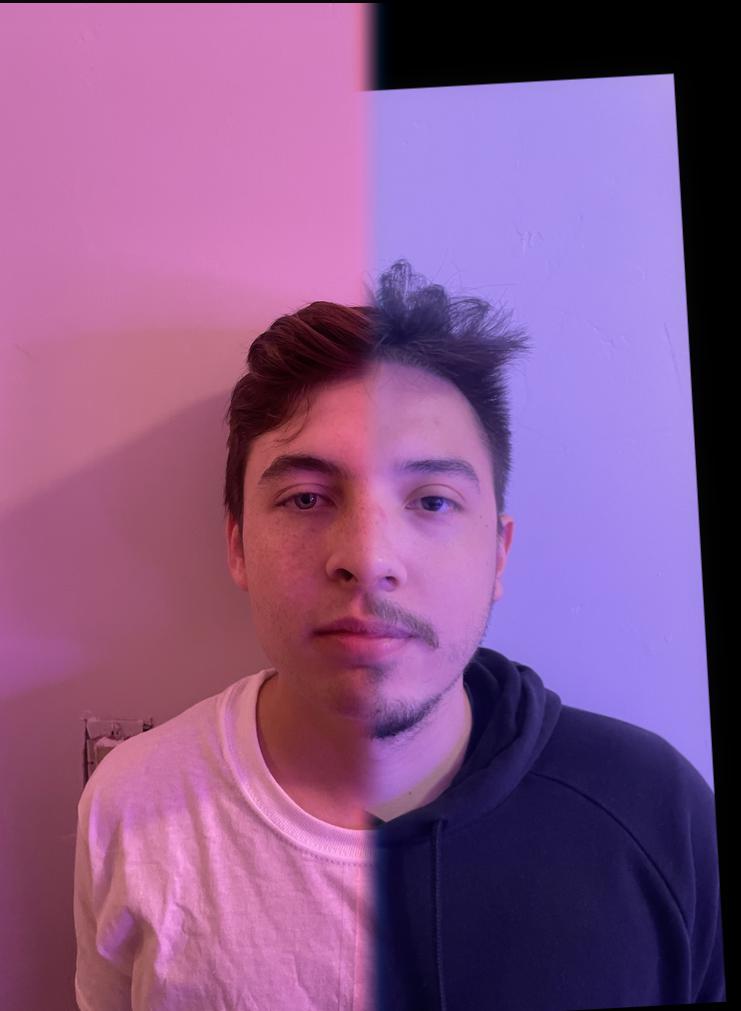
blended (color)
Below is another set of blended images with an irregular mask. I got the snow image from here.
Dumpling
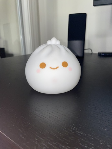
left
Snow
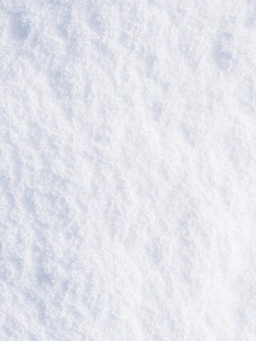
right
Irregular Mask
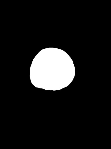
Made with Gimp
Dumpling in the Snow BW
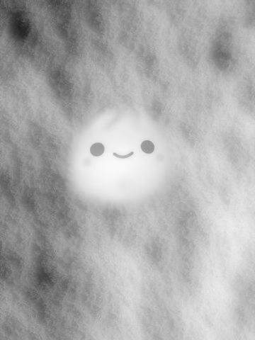
blended (BW)
Dumpling in the Snow
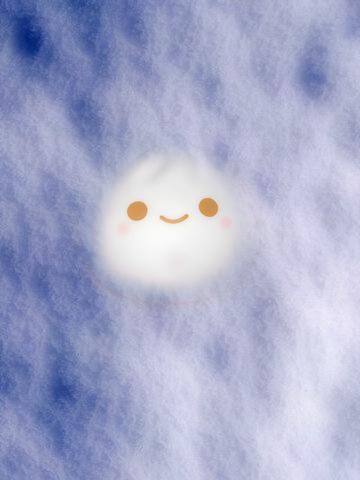
blended (color)
For 2.3/2.4, I used color to enhance the effects of the blending (although sometimes the gray looked better due to differences in brightness/color). The coolest/most interested thing I learned while doing this project is how to conceive images as low and high frequencies and what you can do with images by playing with frequencies. Many of the tools you use with your phone or Photoshop use Gaussian and Laplacian filters and I never even knew (didn't even know images had frequencies to be honest). The results I got from this project were super cool and I already have requests from my girlfriend to blend / hybrid different personal photo combinations. I have a much better understanding of images and how we perceive them. Really cool project!