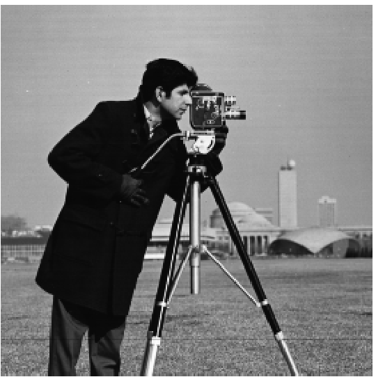
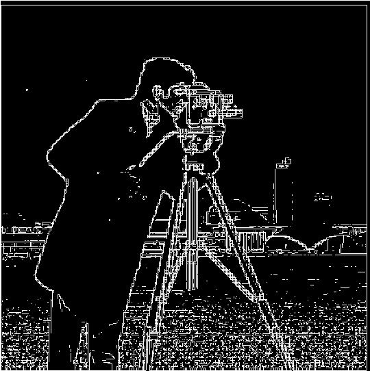
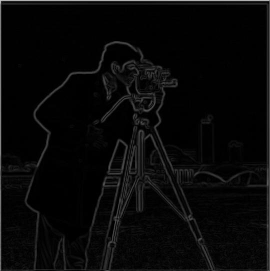
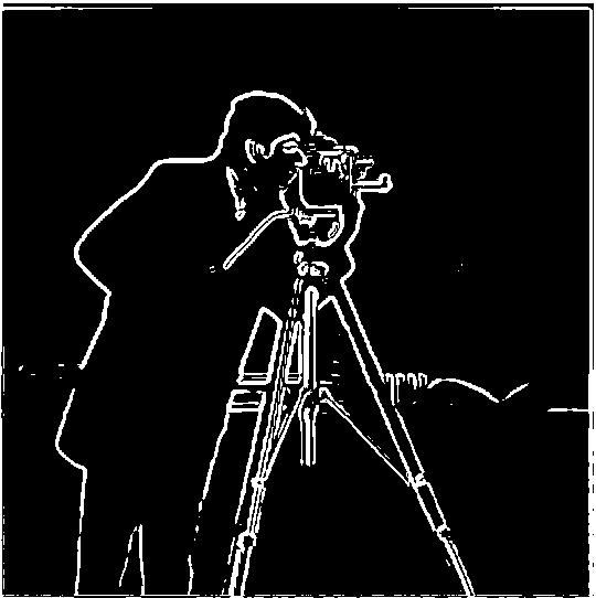
The gradient magnitude computation was done by firstly convolving the image in the X and Y direction with the Dx = [1 -1] and Dy = [1 -1].T matrices respectively. This was equivalent to finding the partial derivatives with respect to X and Y. I then combined these two partial derivatives by taking the magnitude --> (Partial_X^2 + Partial_Y^2)^0.5. The magnitude will be greatest in the areas with the most change and therefore, finding this magnitude is similar to an edge detector as edges have rapid change. To actually turn it into an edge image, I binarized the gradient magnitude image by setting all values above a certain threshhold to 1 and everything below to 0. This threshhold was found simply through trial and error, and as can be seen by the below results, it does work to a certain extent but it is rather noisy because of the noise in the original image.
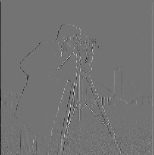
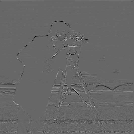
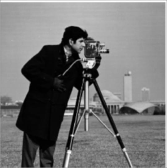
To improve the issues with noise in the previous section, we will now convolve our cameraman image with a Gaussian filter before taking its Partial X and Y derivatives, finding the magnitude, and binarizing. Convolving with a Gaussian filter is essentially blurring the image or smoothening it, and this will remove a lot of the previously seen noise, which should lead to a cleaner edge image.
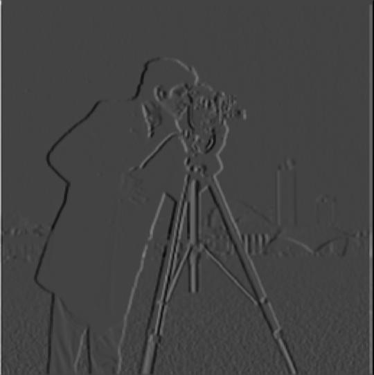
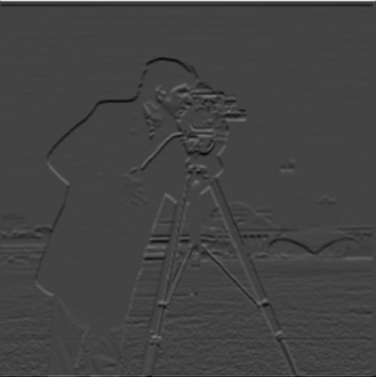
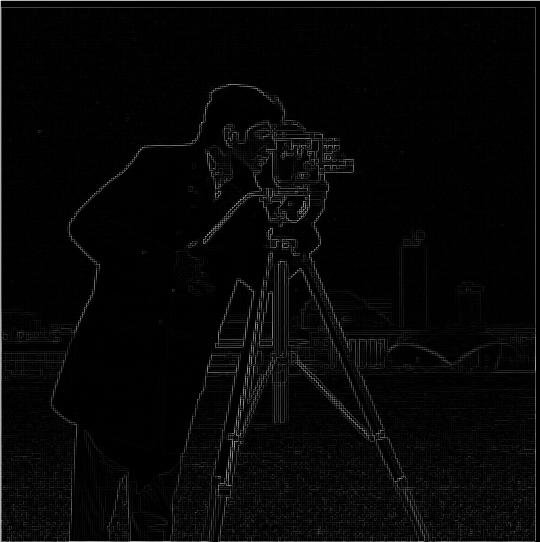
Comparing the Edge image to the one from the previous section, we can see that the lines are a lot smoother and a lot of the noise in the sky and the grass has been removed due to the blurring. Furthermore, the main subject of the image - the cameraman and his camera - is where most of the edges have been defined. However, this has come at the cost of some of the edge detection in the background (in the buildings, etc.) being lost since the blurring process did not preserve the differences in the pixels there. We can also use a second approach to compute this edge image where we first compute the partial X and Y derivatives of the Gaussian filter (by convolving with Dx and Dy) and then convolve the cameraman image with this gradient Gaussian. This will get the same exact result as seen below due to convolving being associative.

To sharpen these images, we create a unsharp mask filter by using the following formula:
unsharp_mask_filter = (1+alpha)*unit_impulse - (alpha*gaussian_filter)
Essentially, this filter takes the unit impulse (the identity filter), adds alpha to its only non-zero entry, and then subtracts away the gaussian filter scaled by alpha. Convolving with this unsharp mask filter will "sharpen" the image as you're obtaining and adding more of the high frequencies into the image. Alpha becomes a parameter for the sharpening (as alpha increases, the more the image is sharpened. It can be seen that with extremely high alpha values, the image looks very artificially sharpened instead of it being a naturally sharp photo. You can see the results for a series of images below:


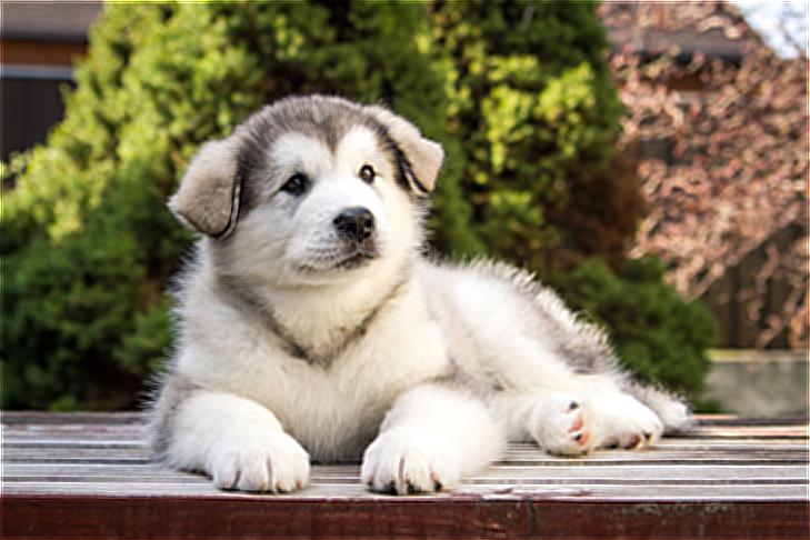
I then tried to take an image, blur it (by convolving it with a Gaussian filter), and then use the unsharp mask filter on the blurred image. All the stages of this process can be seen through the images below. In general, it was found that taking the blurred image back to a sharp one required a much larger alpha value than for the previous images (Alpha = 10). Furthermore, since the high frequencies are removed during the blurring process, using the unsharp mask filter afterwards is not the same as reverting the image to its original version because you have simply lost some of the frequencies to work with. It can be seen that this leads to some artifical effects such as the dog's hair near his back paws being sharpened even though they weren't in the original image due to the depth of field.


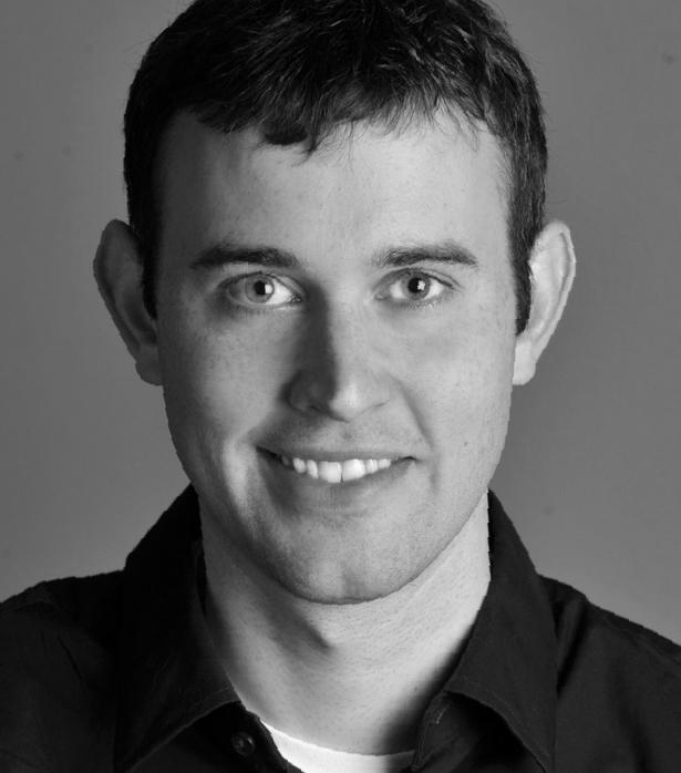
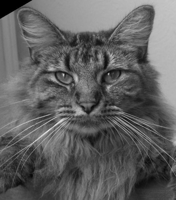
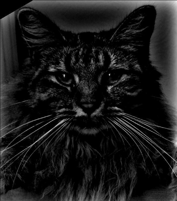
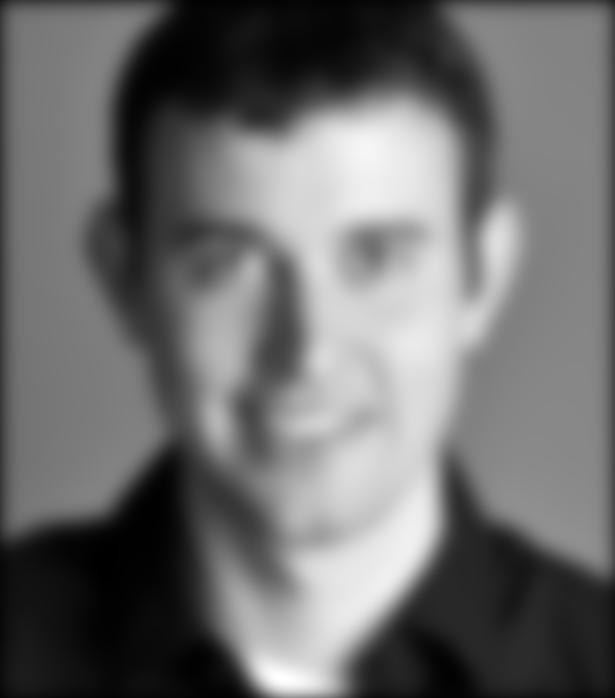
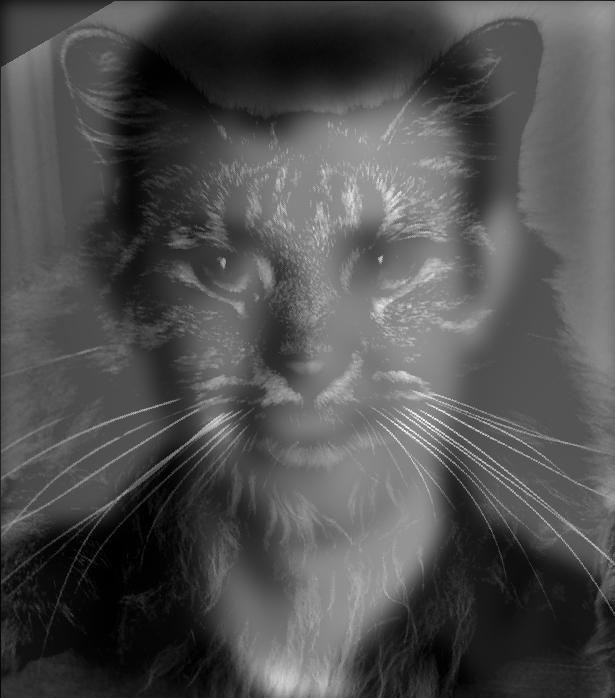
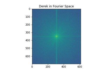
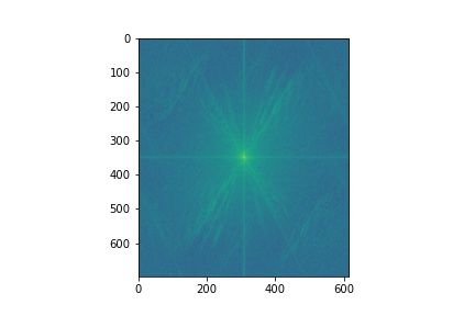
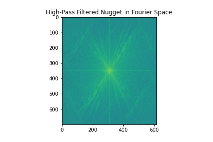
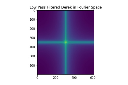
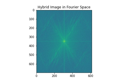
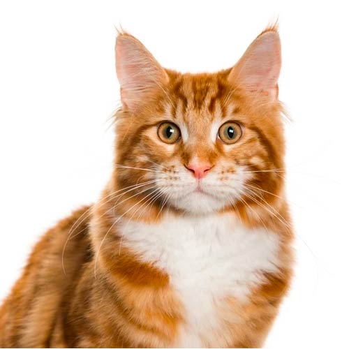
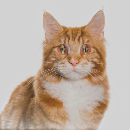
For this part of the project, we try to create 'hybrid images' by applying a high-pass filter to one image and a low-pass filter to another. For the low-pass filter, we convolve the image with a Gaussian filter whereas for the high pass filter, we convolve the image with a Laplacian filter (unit impulse - gaussian). We then add the values of the two images and this should result in an effect where the high-pass image can be seen from closer whereas the low-pass can be seen from further away. I also used the provided alignment code to align the images based on some chosen points (For the cat and Derek, I chose the alignment points as the pupils) so that the effect is more convincing. One change I made was to clip away any values below 0 and above 1 after the respective convolutions.
The respective sigma values were 30 for Nugget and 10 for Derek, with the Kernel sizes being 6 times the set sigma value. A range of kernel sizes and sigma values were tried and these were found to be the most visually succesful.
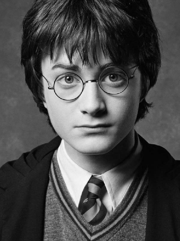
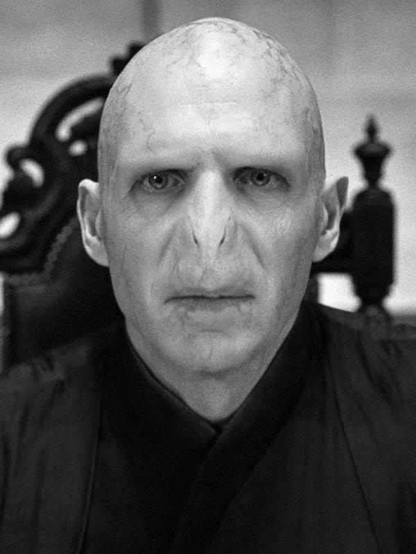
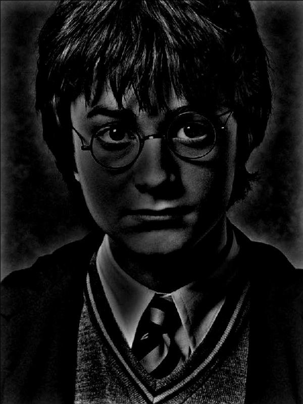
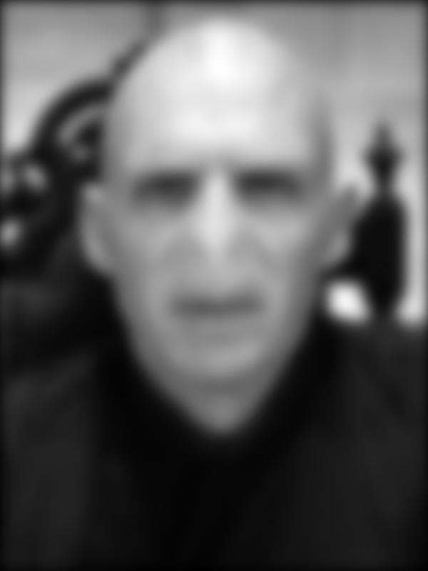
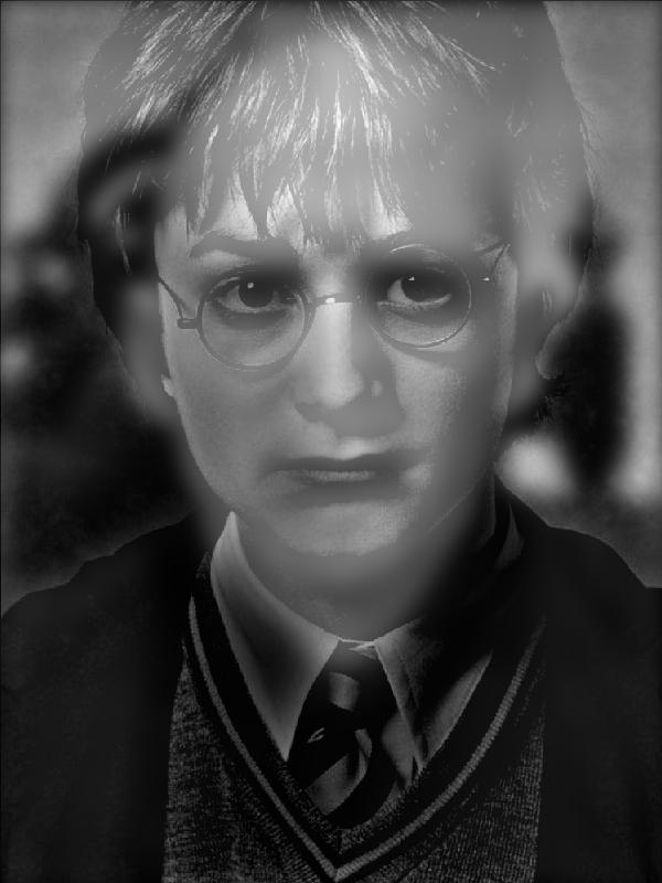
This example also worked fairly well and it was dependent upon choosing images with similar face sizes for both Harry and Voldemort so that the alignment would be more succesful. One shortcoming is that even at distance, Harry's eyes can be seen on Voldy's face and this could be because the low-pass filtered Voldemort is very dark in the eye region.
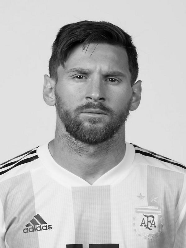
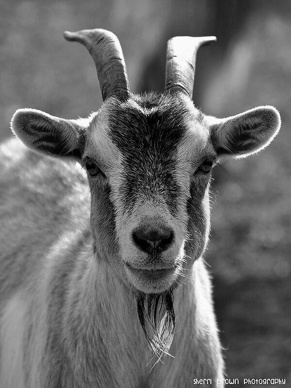
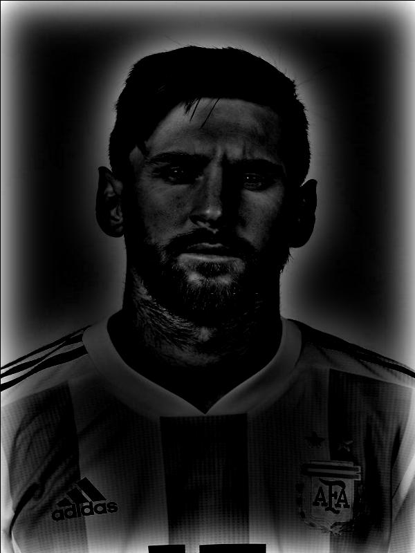
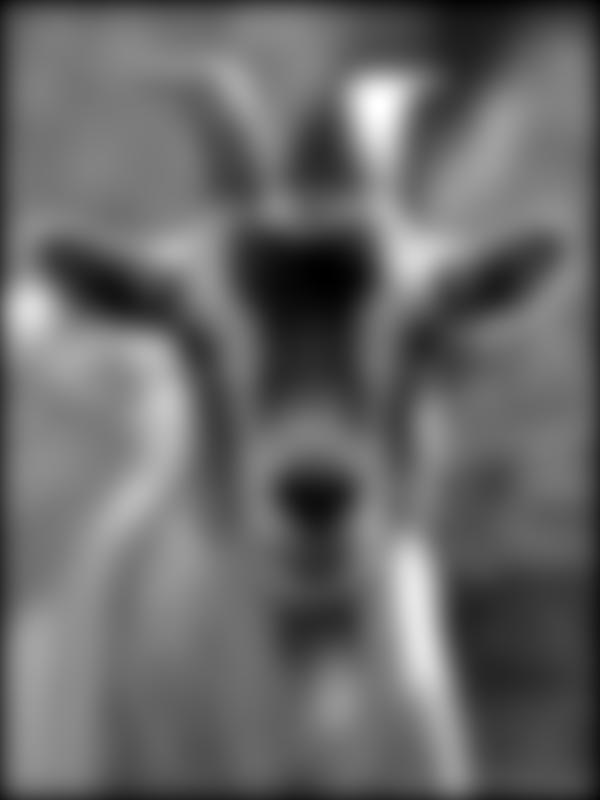
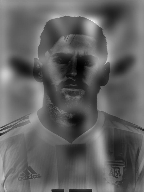
This was a much less successful example because the goat's features can be seen even from a close distance. A variety of things were tried to fix this: Swapping which image was the high-pass and which was the low-pass, increasing the sigma and kernel size so the low-pass image is blurred more, aligning the images more closely. However, the overall effect is still not extremely convincing and this could be because the shapes of the faces are clearly different and the goat's image just being darker to start with, which contrasts with Messi's lighter image.
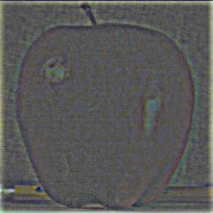
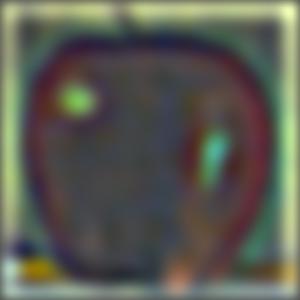
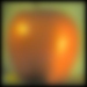
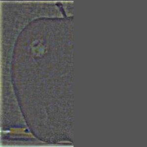
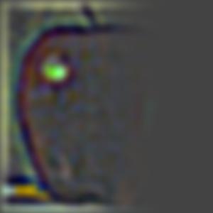
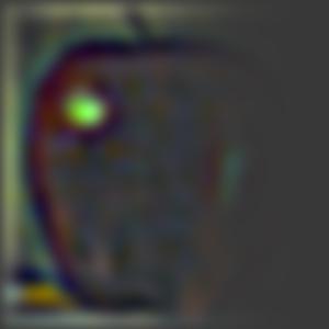
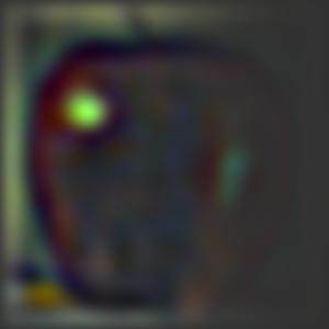
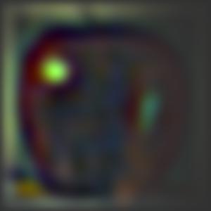
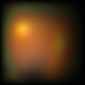
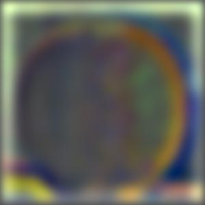
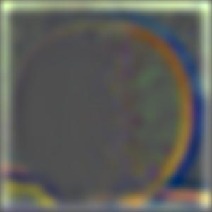
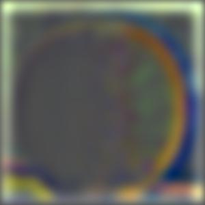
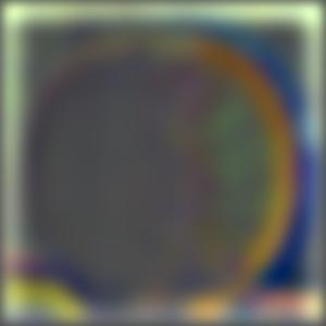
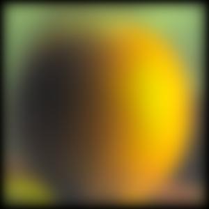
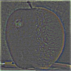
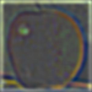
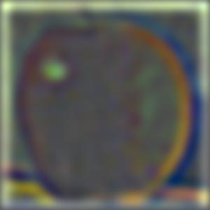
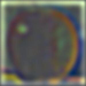
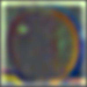
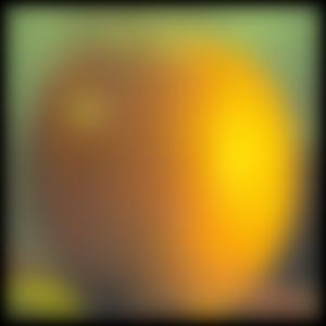
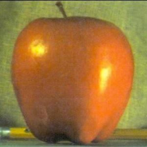
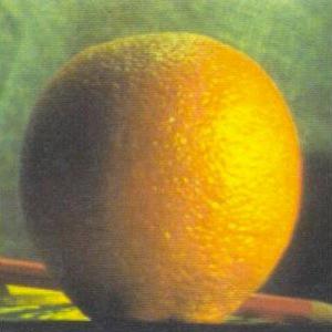
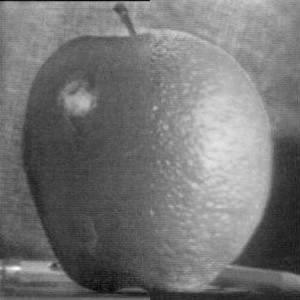
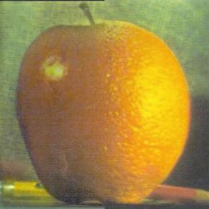
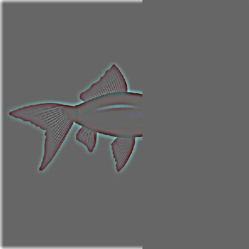
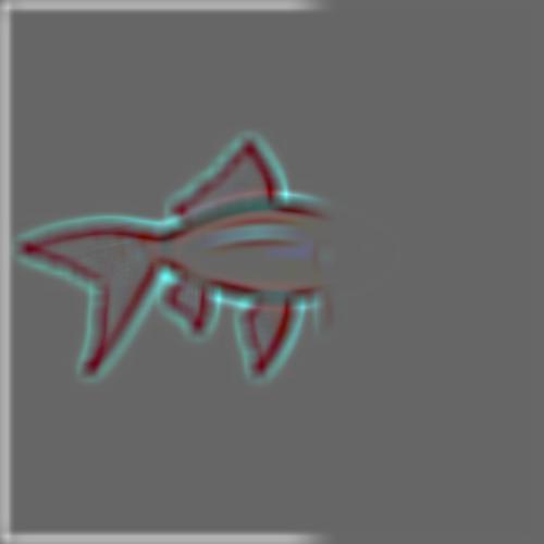
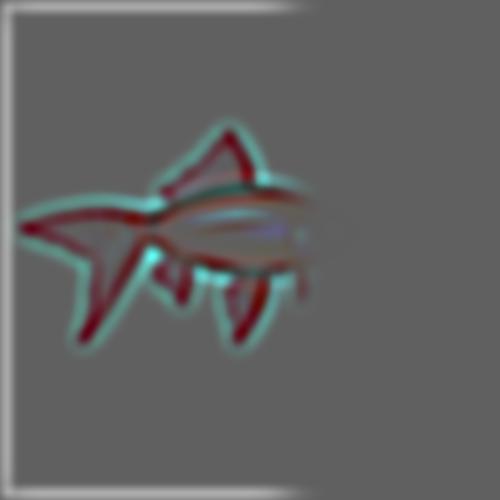
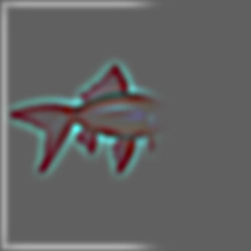
The Gaussian stack was implemented by repeatedly convolving the input image with a Gaussian filter, where each layer represents an additional convolution pass. Therefore, at each layer, the image gets more and more blurred. Between these layers, the size of the image remains the same which is why it is a stack not a pyramind. The Laplacian stack was implemented by taking the difference between sequential Gaussian layers. i.e The first layer of the Laplacian stack is the Gauss_layer_1 - Gauss_layer_2. The last layer of the Laplacian stack is the same as the Gaussian stack, as it is simply the lowest frequencies. Each layer of the Laplacian stack then acts like a Band-Pass filter as it will only capture those specific range of frequencies. For this section, I found a Laplacian stack for the Apple and the Orange respectively, and then masked each layer using the Gaussian stack for the mask (A split black-white image). You can then combined these mask-weighted layers to blend the images at all the different layers. You can see that for the higher frequencies, the spline is very visible whereas for the lower frequencies, it's harder to see because of the blurring of the mask. (Lower layer numbers correspond to higher frequencies, whereas higher layer numbers are the lower frequencies)
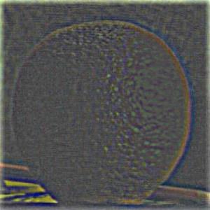
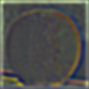
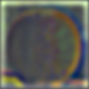
Laplacian Stack Layers for Apple Image:
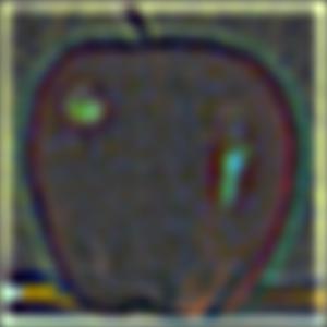
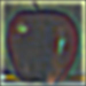
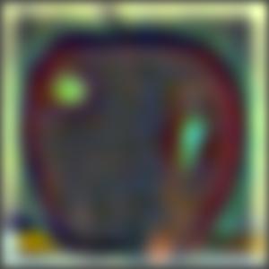
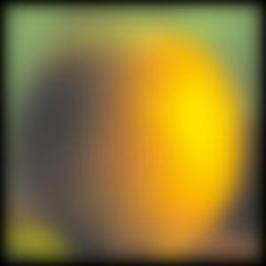
Masked Laplacian Stack Layers for Apple Image:
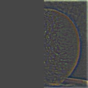
Laplacian Stack Layers for Orange Image:

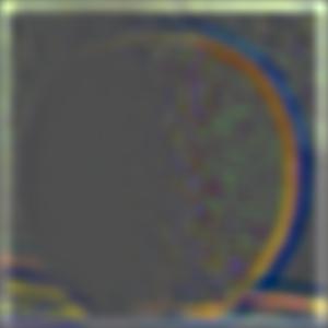
Masked Laplacian Stack Layers for Orange Image:
Blending at Different Frequency Levels:
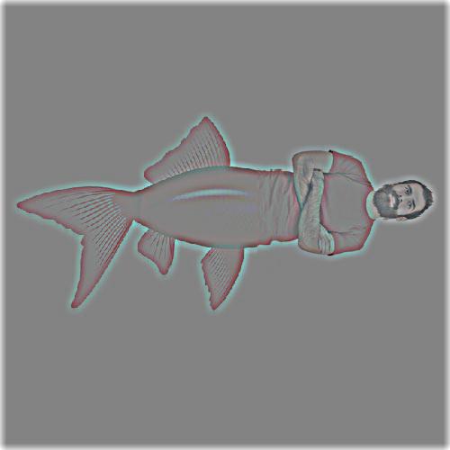
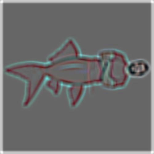
For the Multiresolution blending, you just take all the different blended layers (from the previous section), and add them all up to create one blended image at many resolutions. Below it can be seen in greyscale and color (for extra credit). In my opinion, the color version is much more satisfying as you can see the transition between the fruits and the effect of the gradual blend more clearly.

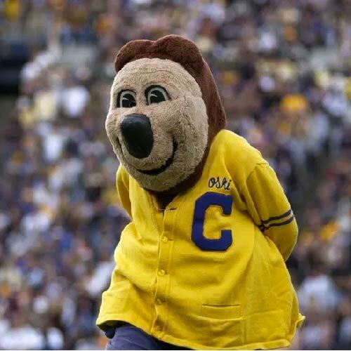
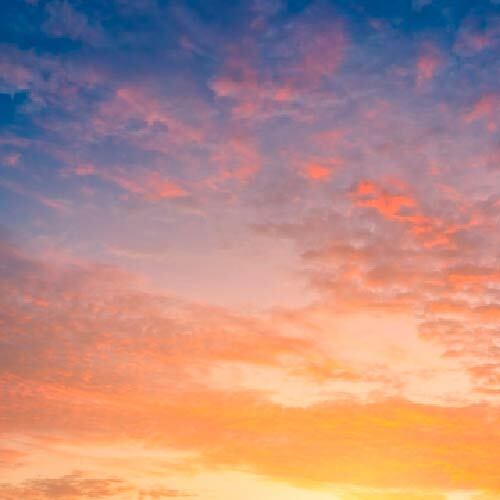
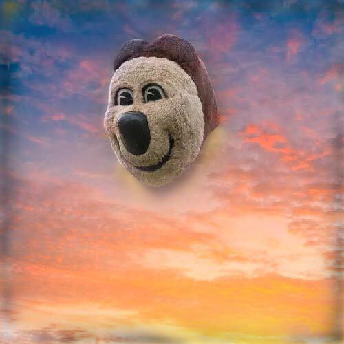
This blend attempt taught me that both images must be compatible in their color palette and lighting. Here, Oski's face is mostly brown whereas the sky around him is blue/purple which is why the blend is a bit more jarring.

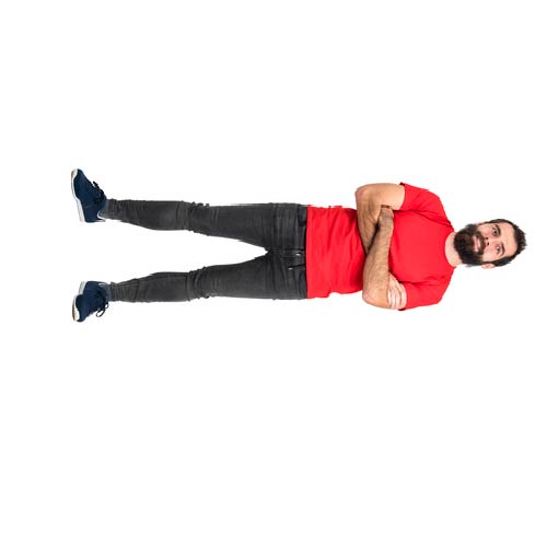
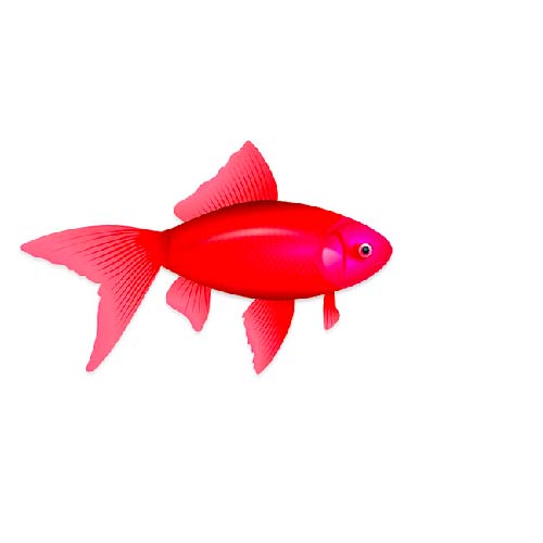

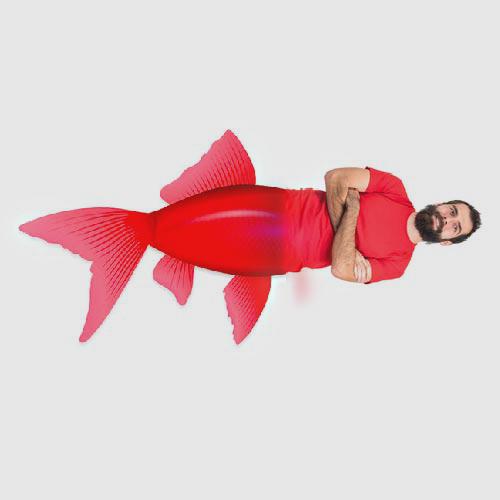
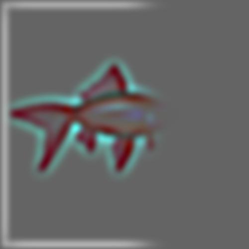
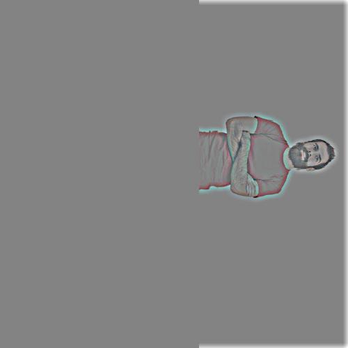
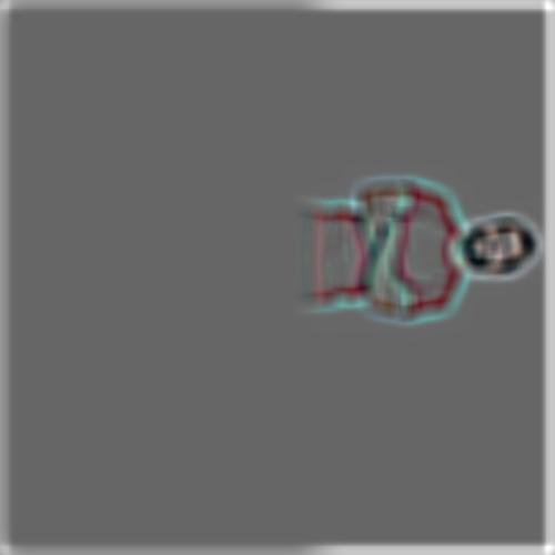
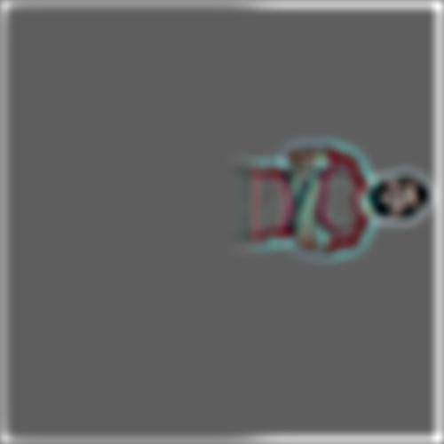
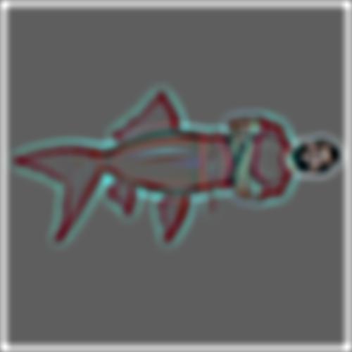
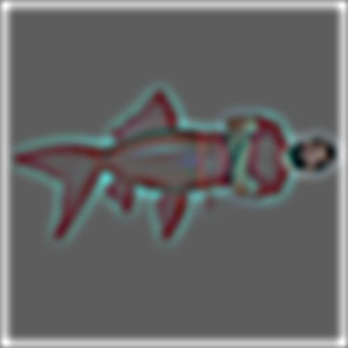
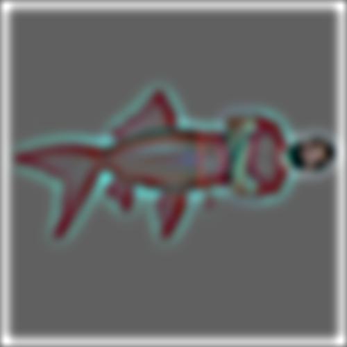
You can see that on the higher frequencies, the extra fin (below the man's right arm) is not visible because the mask weighting is not as gradual. However, on the lower frequencies, this extra fin becomes more visible because the window size is larger and the image is more blurred. Although this is useful in make the blend more gradual, it also results in this blurred fin artifact in the blended image which is not ideal. This could be fixed through placing the mask more carefully though.


For the extra credit part of this Project, I chose to implement multi resolution blending with color. Multiple examples of this can be seen in the previous section.
I learned a lot through this project, especially because as an amateur photographer, I tend to use Adobe Lightroom a lot. Effects that I commonly play with such as the Sharpening and Blurring filter are so much more interesting to me now because I know the actual computations that are behind them. However, the most important thing that I learned in this project is that even with all these mathematical computations, human input and qualitative evaluation is still needed quite often. For example, I implemented a multi resolution blending algorithm but the way I chose the proper kernel size and sigma values was just by trying out a bunch of different ones and seeing which looked best to my eye. This was the same approach I used to decide the alpha values for my unsharp mask filter. Although computers are very impressive in terms of how fast they can do these computations, humans are still needed to decide what 'looks best'.
Cameraman --> Provided through project spec
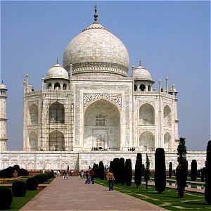
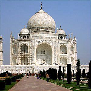
Taj Mahal --> Provided through project spec
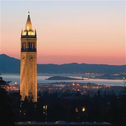
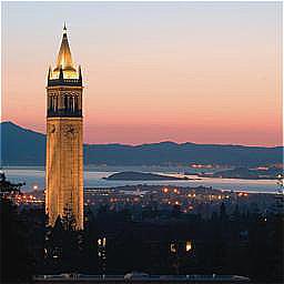
Campanile --> https://twitter.com/ucb_campanile
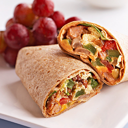
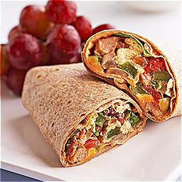
Burrito --> https://www.savemart.com/recipes/breakfast-burritos/11362
Puppy --> https://www.thepedigreepaws.com/dog-breeds/alaskan-malamute
Derek and Nugget --> Provided through project spec
Harry Potter --> https://www.irishtimes.com/culture/books/harry-potter-is-there-a-less-appealing-fictional-character-1.3170112
Tom Riddle --> https://harrypotter.fandom.com/wiki/Tom_Riddle
Messi --> https://www.biography.com/athlete/lionel-messi
Goat --> https://fineartamerica.com/featured/goat-headshot-sherri-brown.html
Apple and Orange --> Provided through Course Spec
Oski --> https://www.dailycal.org/2016/04/01/oski-no-longer-cals-mascot/
Sunset Sky --> https://www.istockphoto.com/photos/sunrise-sunset
Cat Headshot --> https://www.shutterstock.com/image-photo/close-maine-coon-looking-camera-isolated-635622530
Eye of Sauron --> https://www.vhv.rs/viewpic/hoTThT_eye-of-sauron-transparent-hd-png-download/
Fish --> https://www.carlswebgraphics.com/fish.html
Man in Red Shirt --> https://fr.123rf.com/photo_55148486_rire-homme-barbu-avec-le-chapeau-en-regardant-la-cam%C3%A9ra-corps-plein-longueur-portrait-isol%C3%A9-sur-fond-bla.html