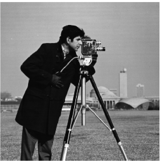
Cameraman Image
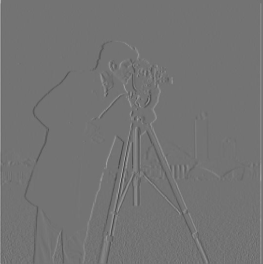
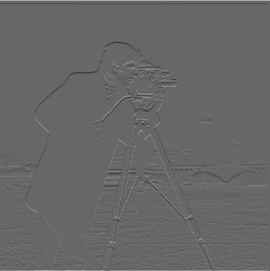
Edge detection is an essential part of image processing. We can find edges where color/brightness change drastically. To get partial derivatives of the cameraman image, I convolved the image with derivative Dx = [1, -1] and Dy = [[1], [-1]]. The resulting two images illustrate how drastic the image is changing horizontally and vertically.
Cameraman Image
| Dx | Dy |
|---|---|
 |
 |
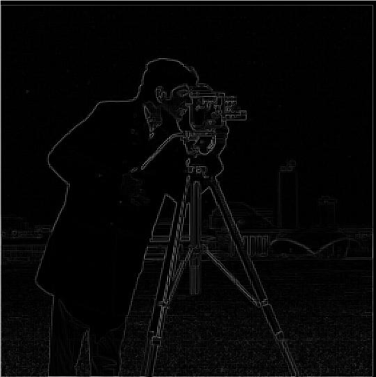
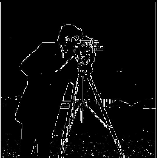
To get a sense of how fast it's changing overall, I computed the gradient magnitude of the image by taking the square root of the sum of its two squared partial derivatives. I then binarize the gradient magnitude image by picking the threshold value 0.2. We see that the binarized image looks a lot clearer than the unbinarized one.
| Gradient Magnitude Image | Gradient Magnitude Image with Threshold |
|---|---|
 |
 |
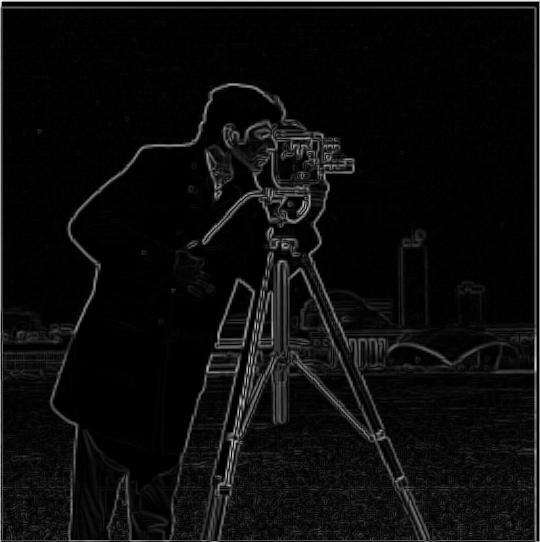
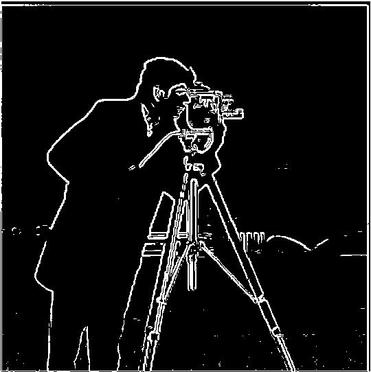
We can see that the images from part1.1 still contain a lot of noise. We can remove noise by using a low pass filter(the Gaussian filter) on the image. We first blur the original image with the Gaussian filter(kernel size = 3, sigma = 1) and then apply calculate the gradient magnitude to find edges. To make the gradient magnitude image sharper, I use threshold value 0.1 here to binarize the image. We can see a significant improvement in the image quality here! Most noise in the image is removed.
| Naive Gaussian filtered Gradient Magnitude Image | Naive Gaussian filtered Gradient Magnitude Image with Threshold |
|---|---|
 |
 |
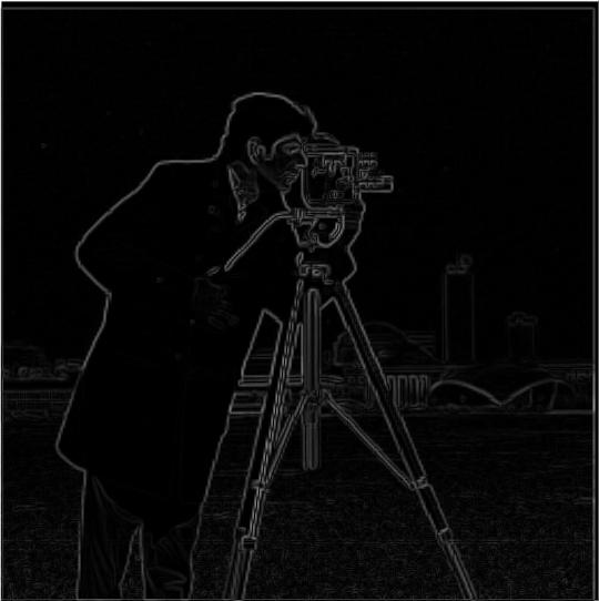
Convolution has a nice associative property, so we can calculate the derivatives of gaussian filter first and then convolve with the image. As a result, we are only performing one convolution instead of two! By comparing the results below to the previous results, we can see that the images are identical but we are getting a computation speed boost!
| Single Convolution Gaussian filtered Gradient Magnitude Image | Single Convolution Gaussian filtered Gradient Magnitude Image with Threshold |
|---|---|
 |
 |
In the last section, we see that Gaussian filter can blur images because they are low-pass filters that retain low frequencies in images. If we subtract the low frequencies from an image, we will get the high frequency of an image, which are the sharp features. Then we can add the high frequency part back to the original image to "sharpen" an image. Here I will demonstrate two ways to implement this procedure:
Here I use alpha=5(adding 5 times the high frequency portion back to the original image) and Gaussian filter with kernel size = 3, sigma = 1.
In below, you can see that the naive implementation and the single convolution implementation both give identical results!
| Original Image | Blurred Image |
|---|---|
 |
 |
| Naive Sharpened Image | Single Convolution Sharpened Image |
|---|---|
 |
 |
Below is my attempt to sharpen a cute german shepherd image hehehe:

German Shepherd
| Blurred German Shepherd Image | Sharpened German Shepherd Image |
|---|---|
 |
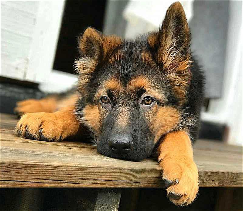 |
I love the sharpened image more than the original one because the features look sharper and we can see a better contrast between the dog and the background. In addition, we can see the tiny details(ex. furs on the paws) better!
The SIGGRAPH 2006 paper by Oliva, Torralba, and Schyns presented some hybrid images that look different when viewed at different distances. The basic idea is that high frequency tends to dominate perception when it is available, but, at a distance, only the low frequency (smooth) part of the signal can be seen. By blending the high frequency portion of one image with the low-frequency portion of another, you get a hybrid image that leads to different interpretations at different distances. We can use this fact to create cool images!!
Below I'll illustrate the process through frequency analysis.
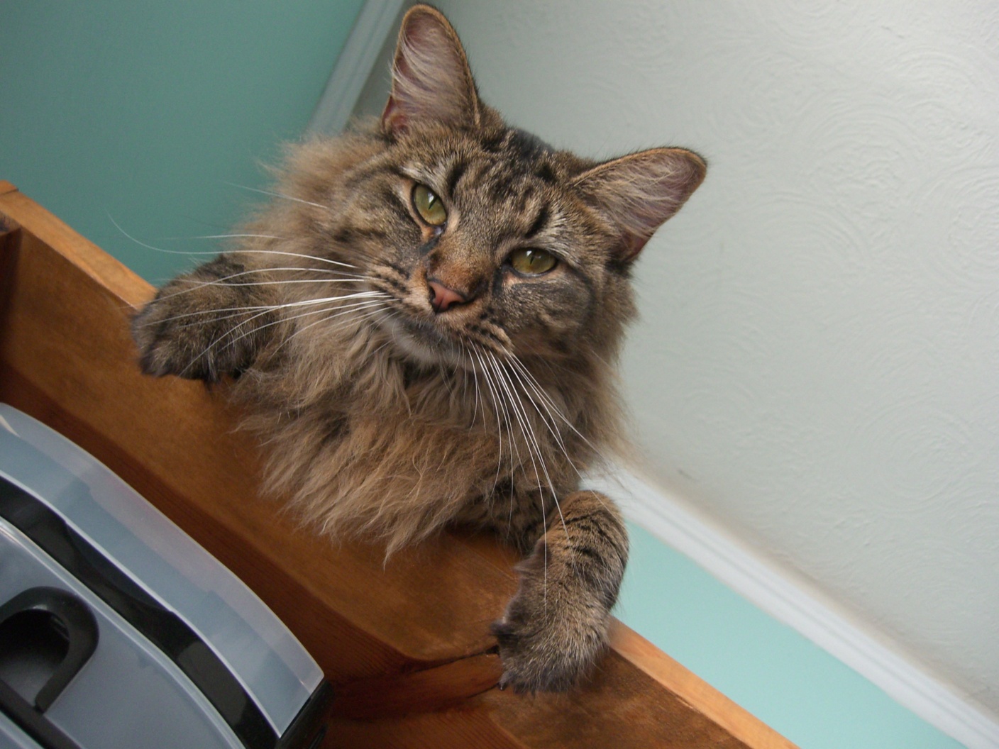
| Derek | Derek Image Frequency |
|---|---|
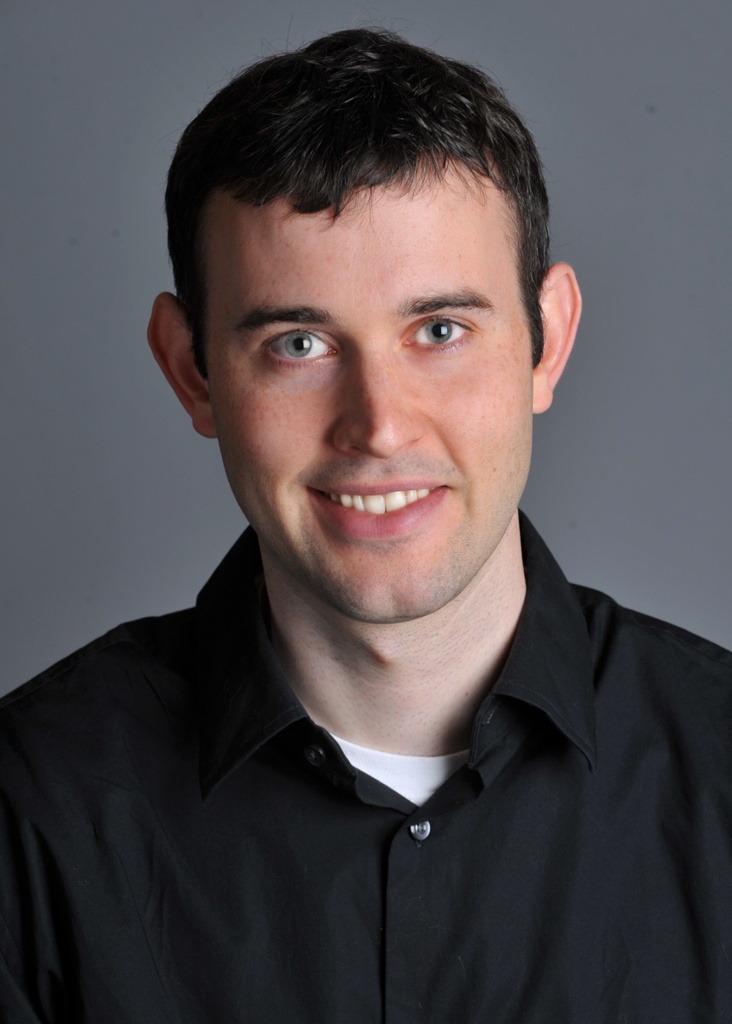 |
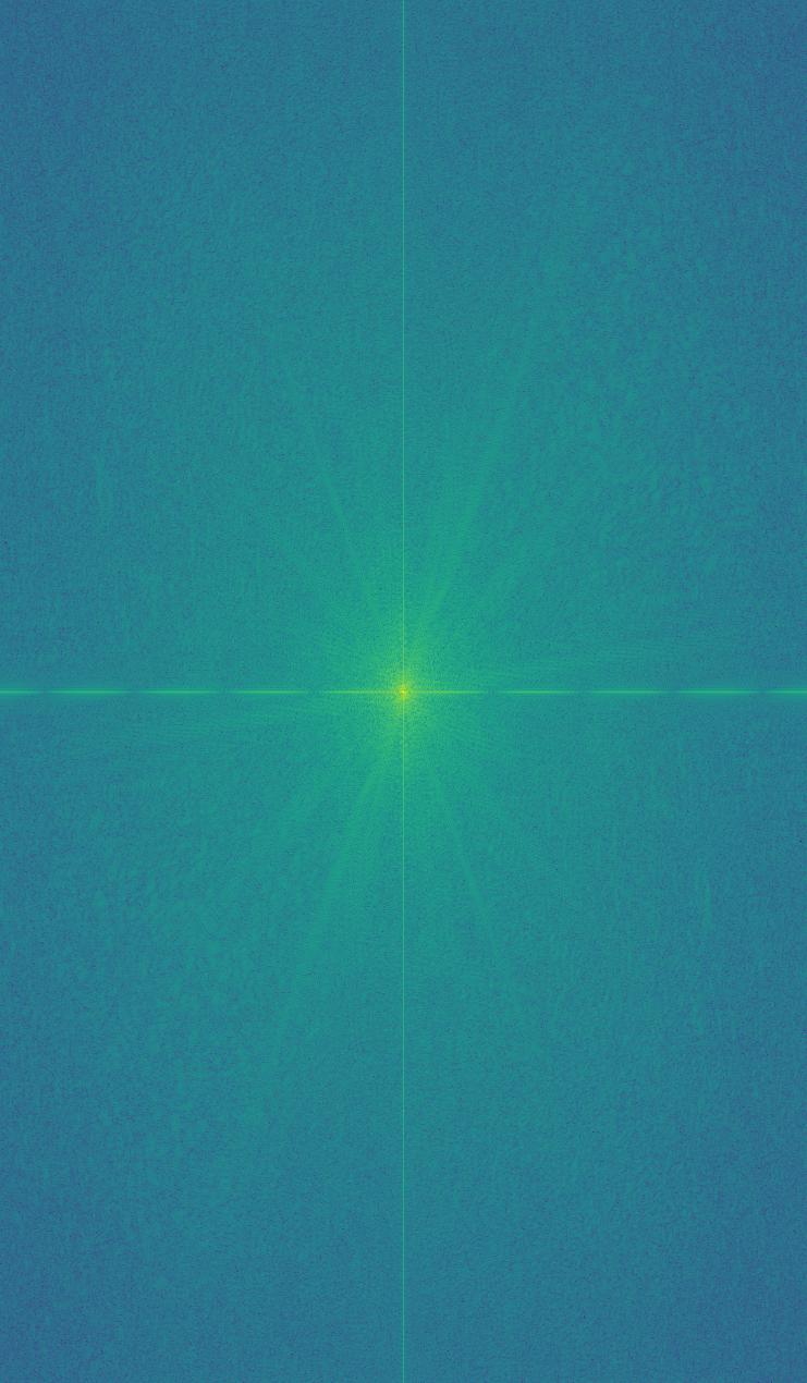 |
| Nutmeg | Nutmeg Image Frequency |
|---|---|
 |
 |
| Low Pass Filter | Low Pass Filter Frequency |
|---|---|
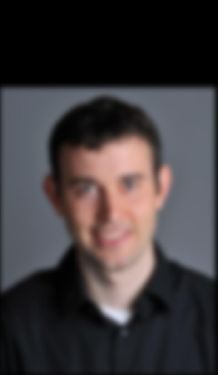 |
 |
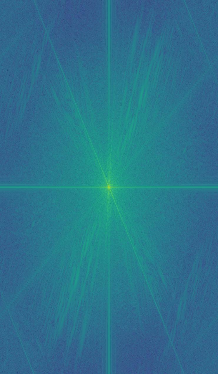
| High Pass Filter | High Pass Filter Frequency |
|---|---|
 |
 |
| Hybrid Image | Hybrid Image Frequency |
|---|---|
 |
 |
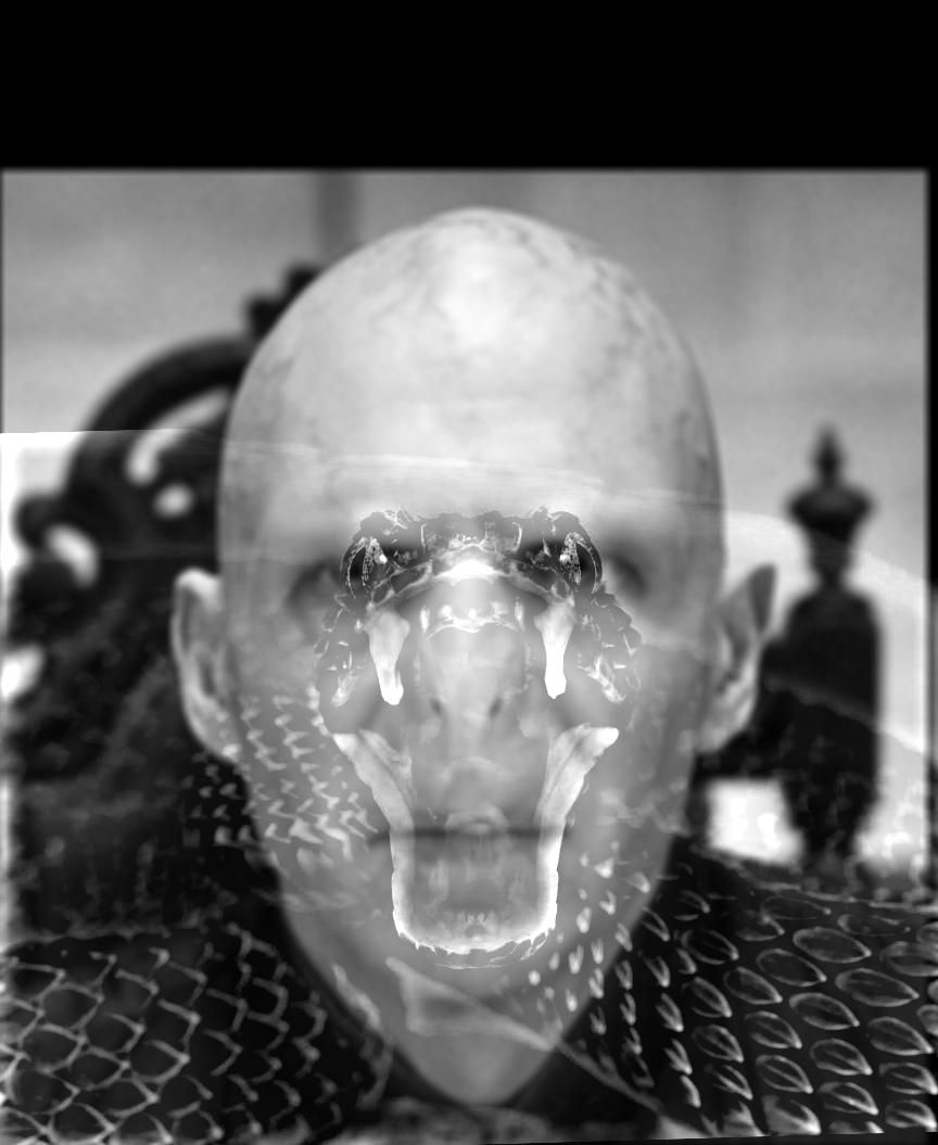
Here's another cool image I created!!
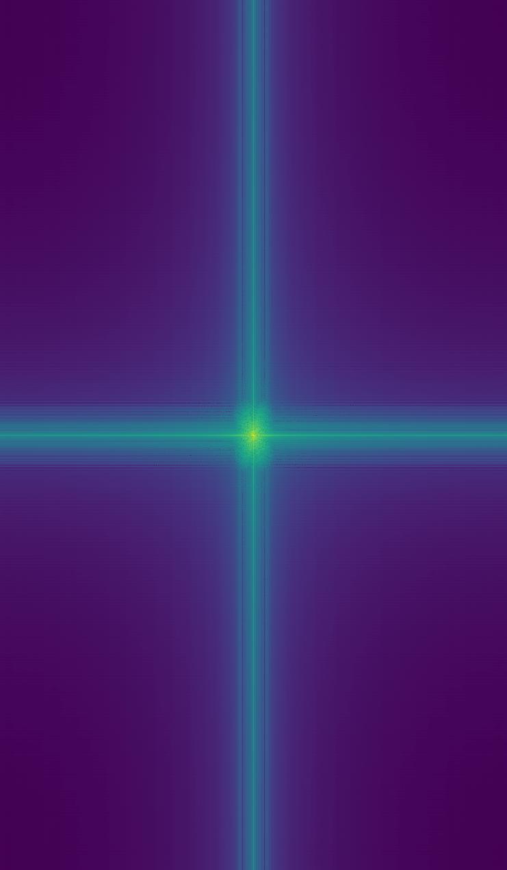
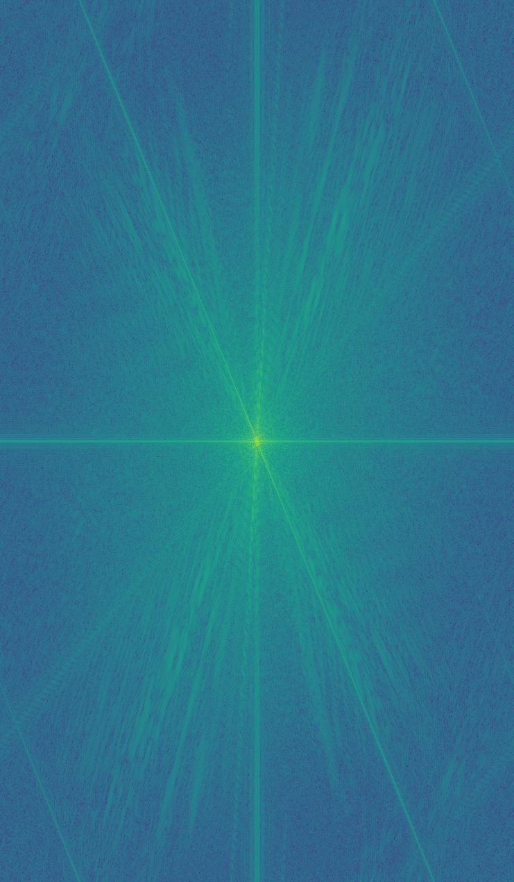
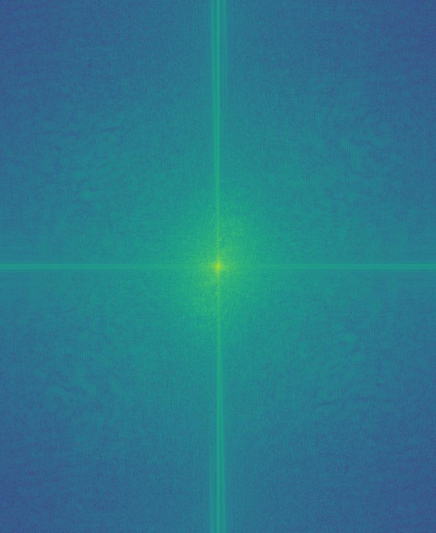
| Voldemort | Voldemort Image Frequency |
|---|---|
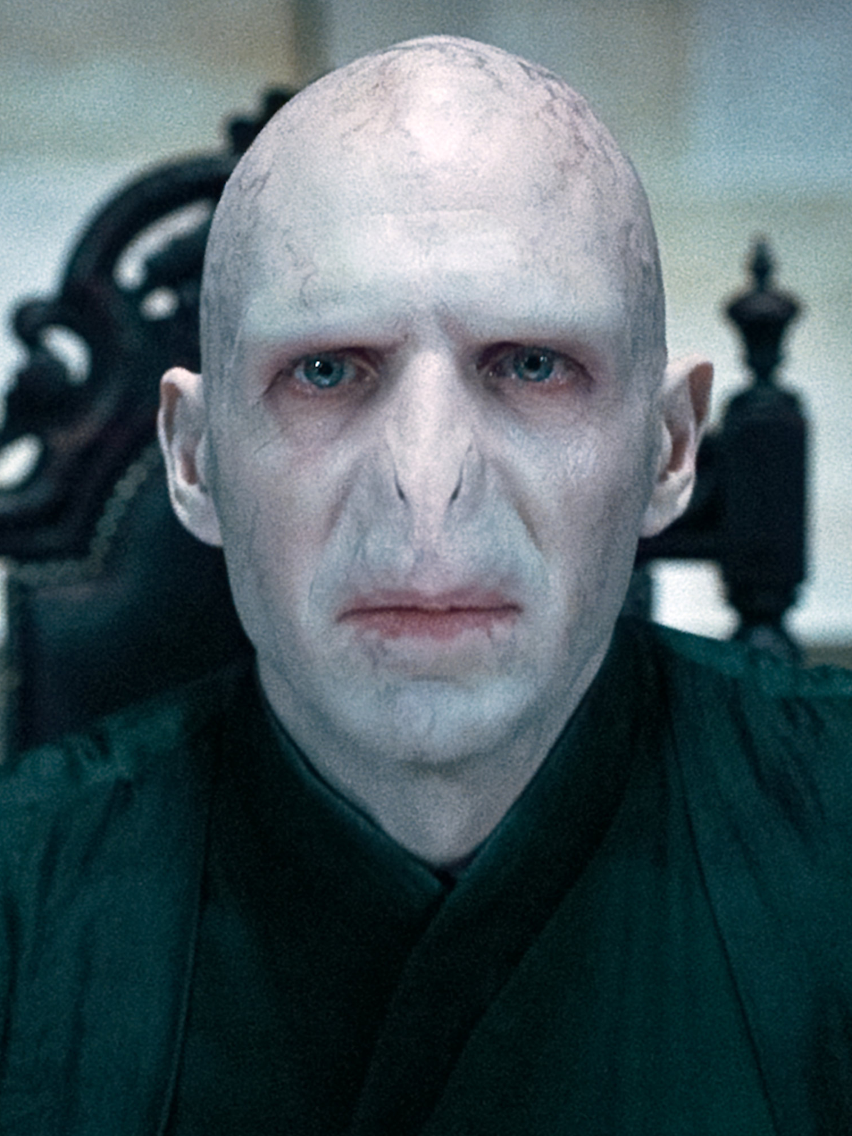 |
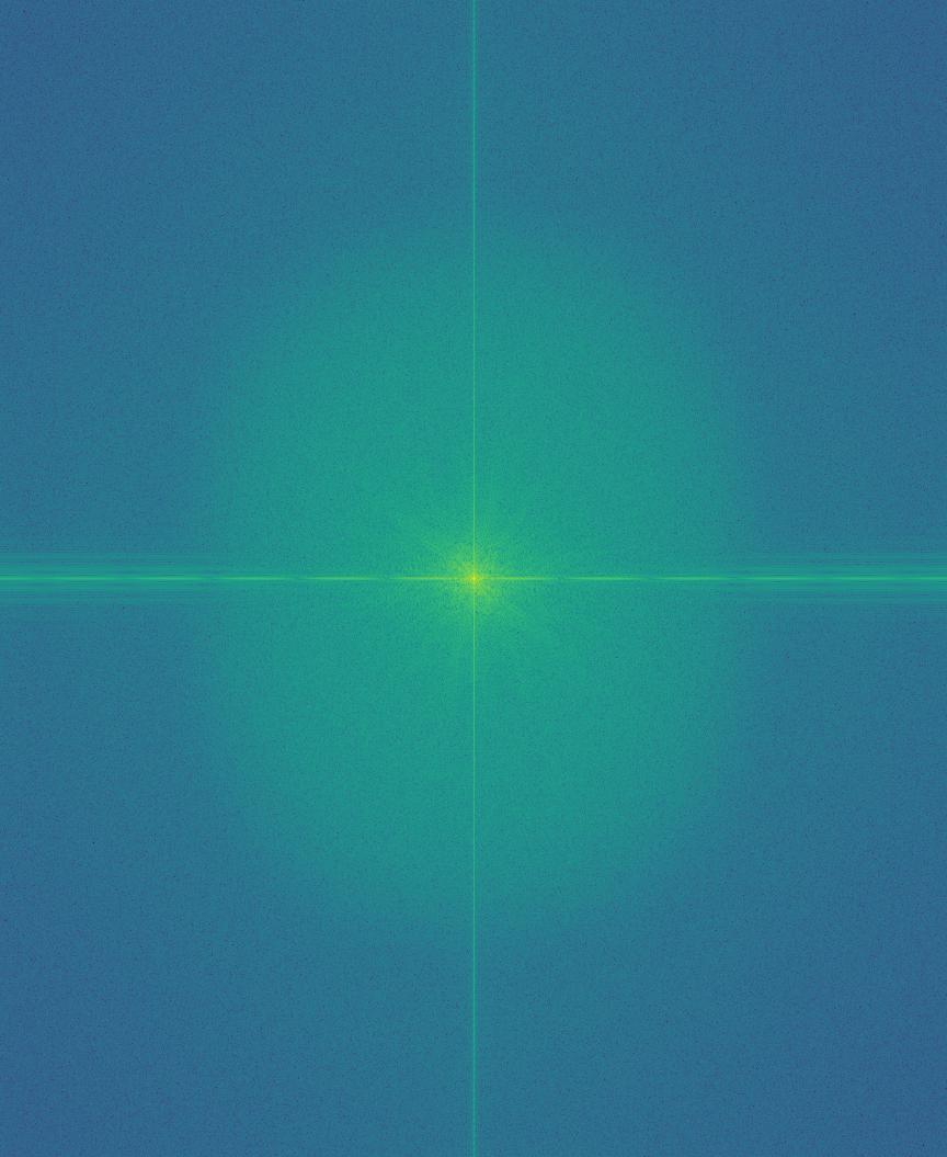 |
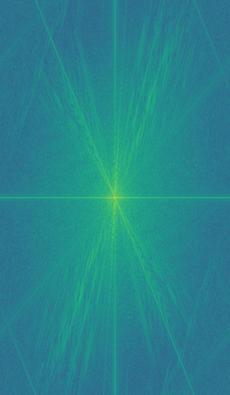
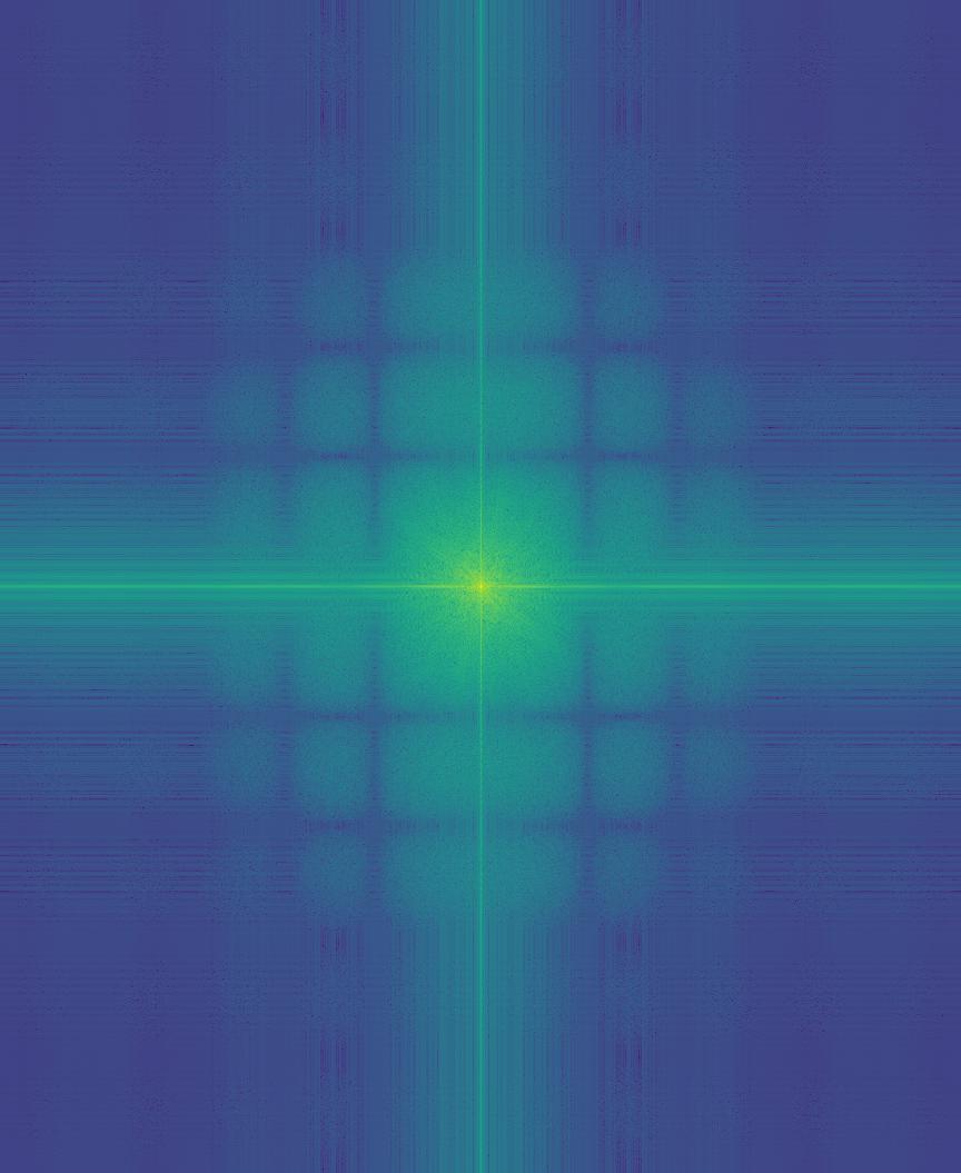
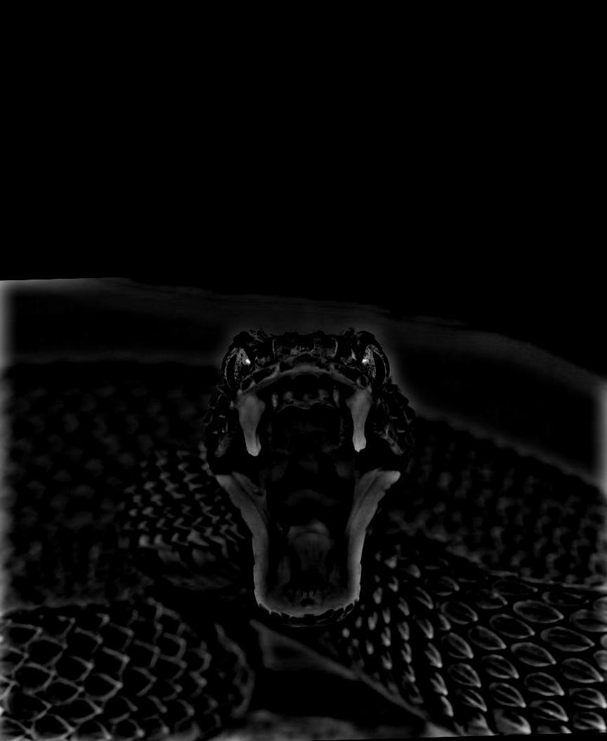
| Snake | Snake Image Frequency |
|---|---|
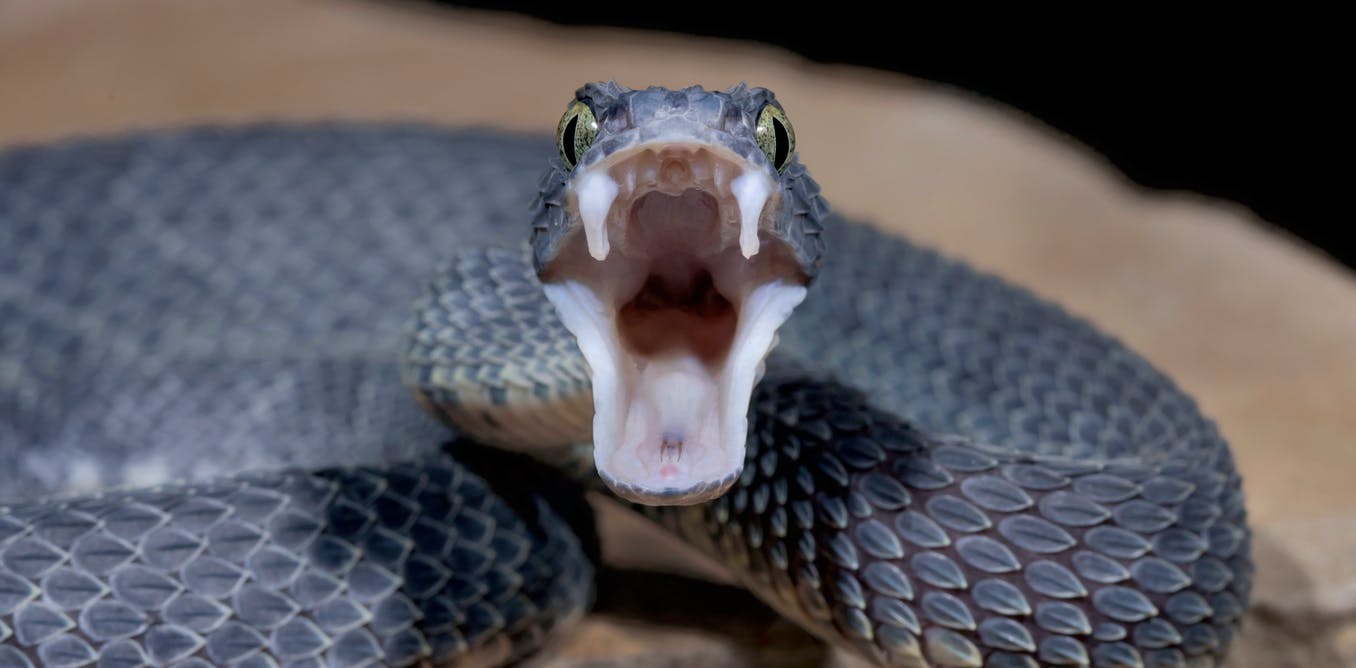 |
 |
| Low Pass Filter | Low Pass Filter Frequency |
|---|---|
 |
 |
| High Pass Filter | High Pass Filter Frequency |
|---|---|
 |
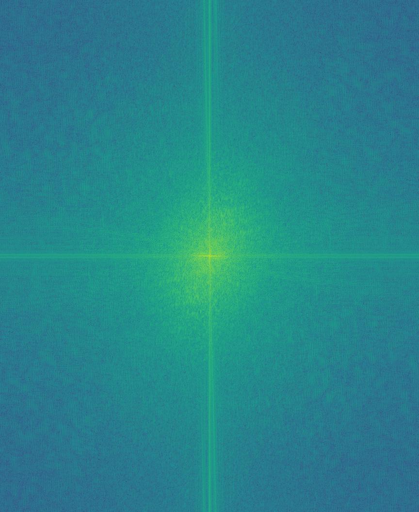 |
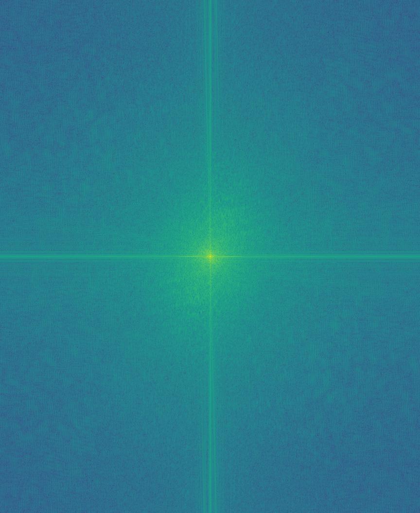
| Hybrid Image | Hybrid Image Frequency |
|---|---|
 |
 |
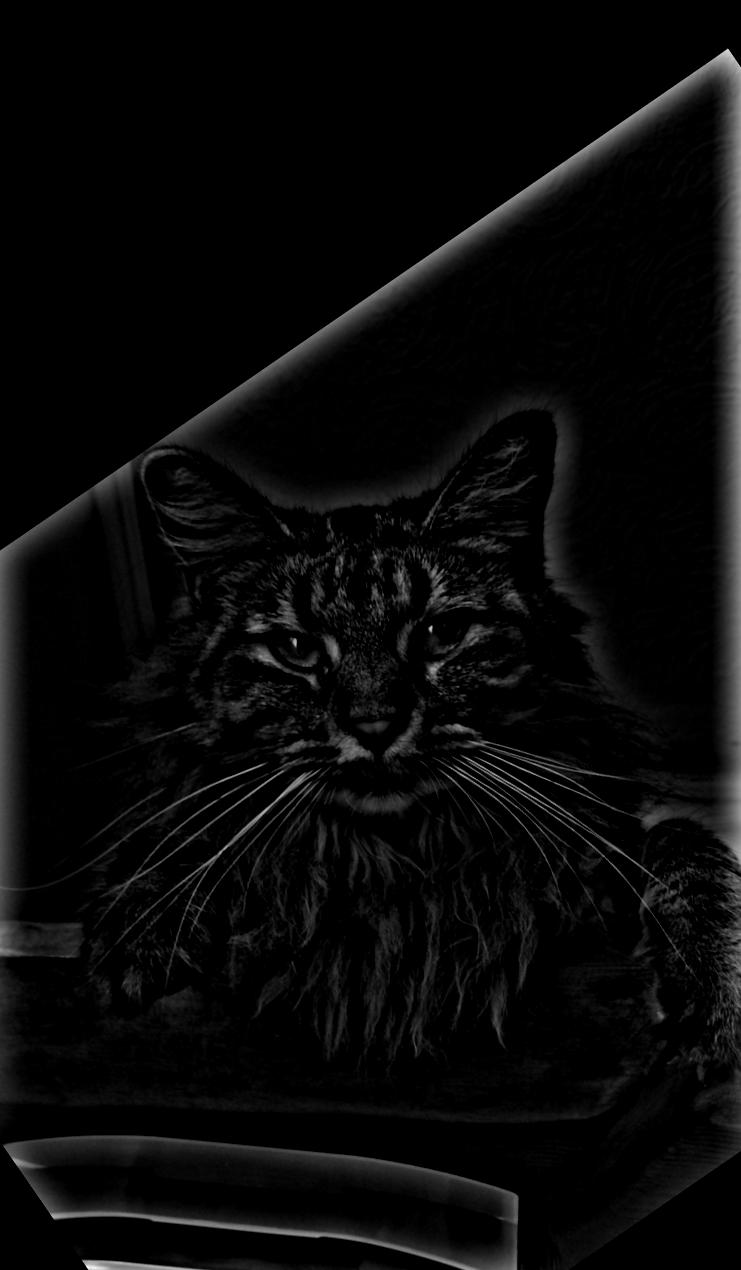
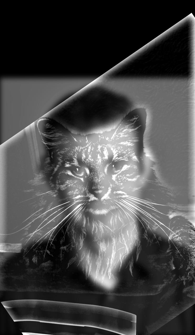
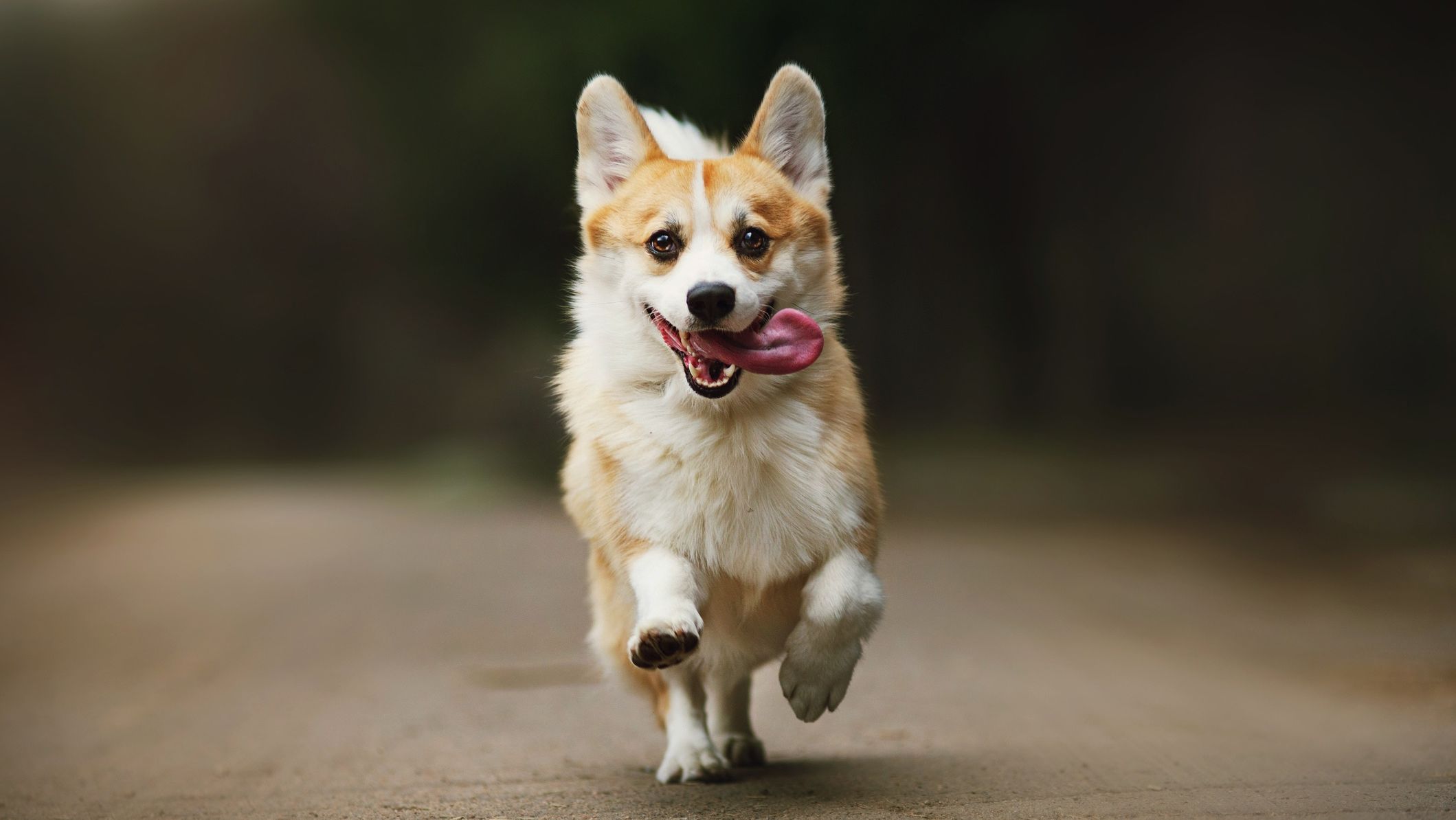
| Corgi | Cat |
|---|---|
 |
 |
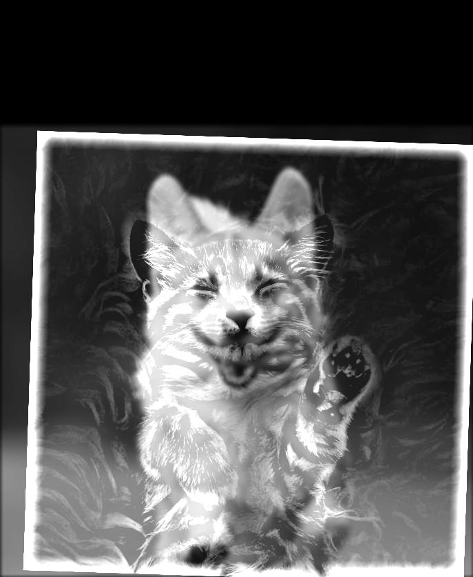
Hybrid Image
Reason for failure: I was attempting to fuse two cute pictures together but the end result just looks weird and creepy :((
I used color to enhance the effect. I found that it works better to use colored low-frequency component and grey-scale high-frequency component!
| Derek+Nutmeg Grey Image | Derek+Nutmeg Colored Image |
|---|---|
|
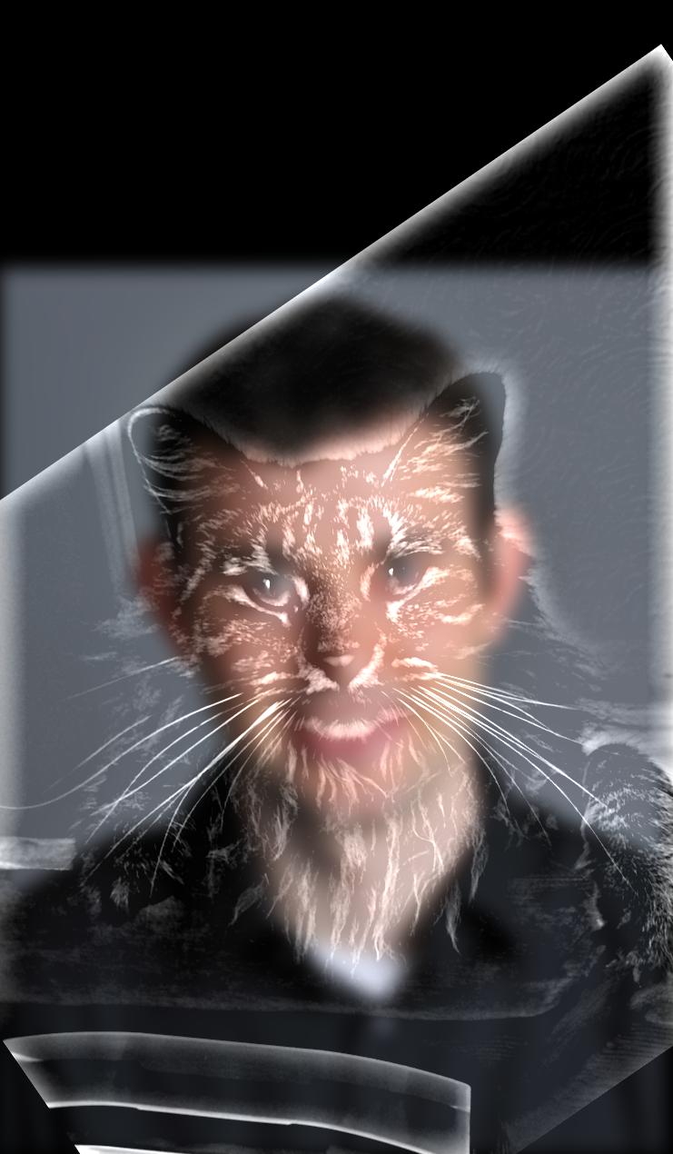 |
| Voldemort+Snake Grey Image | Voldemort+Snake Colored Image |
|---|---|
|
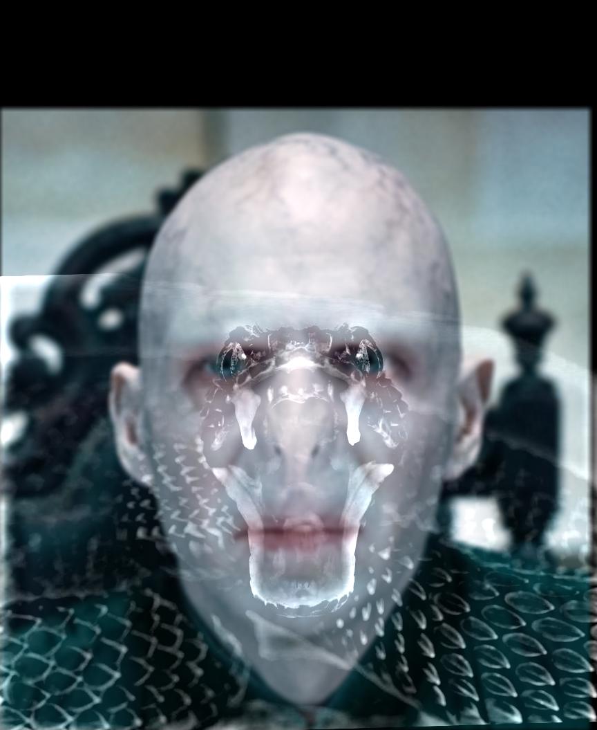 |
| Corgi+Cat Grey Image | Corgi+Cat Colored Image |
|---|---|
|
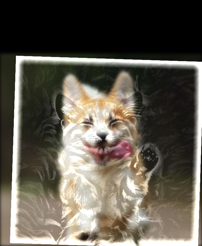 |
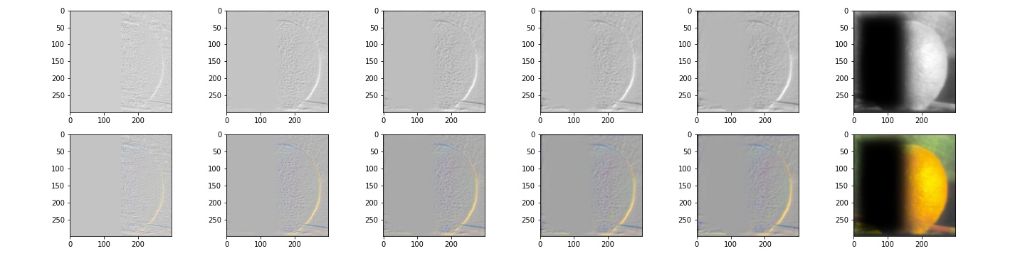
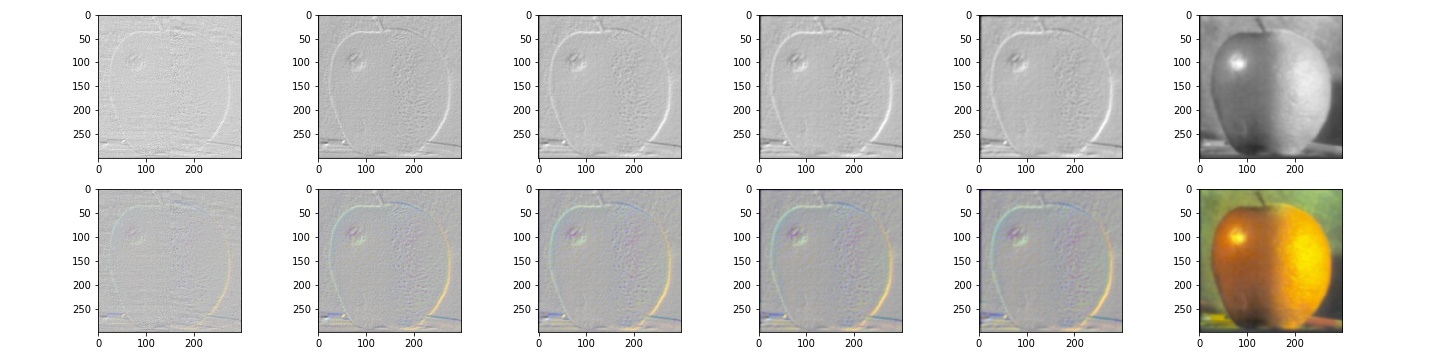
Gaussian Stacks: We start from the original image and apply Gaussian filter sequentially to each level to obtain next level's image.
Laplacian Stacks: we take the difference between any consecutive Gaussian layers to calculate Laplacian layers, and the last layer is the same as the last layer of the Gaussian stack.
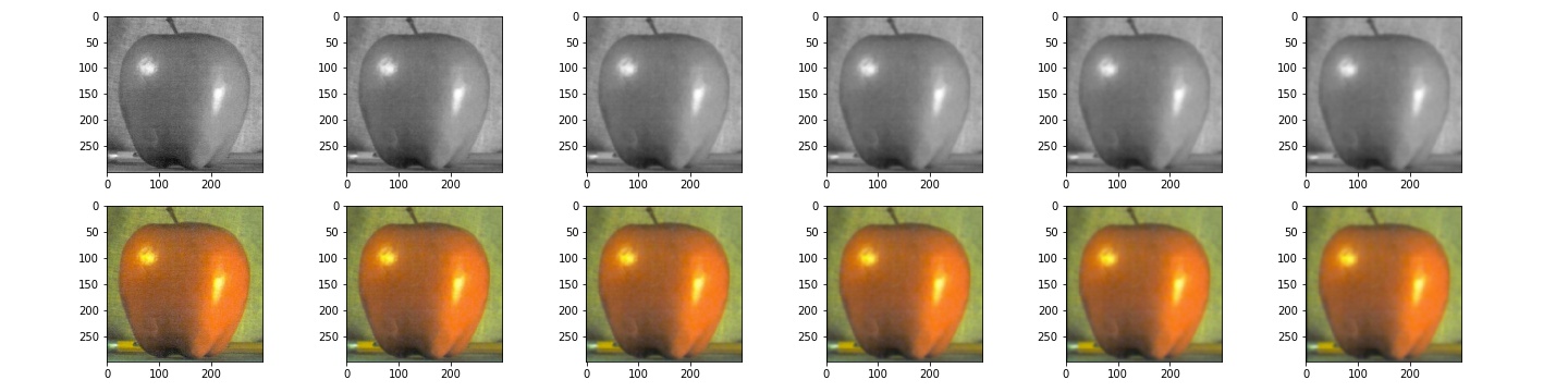
Apple Gaussian Stack
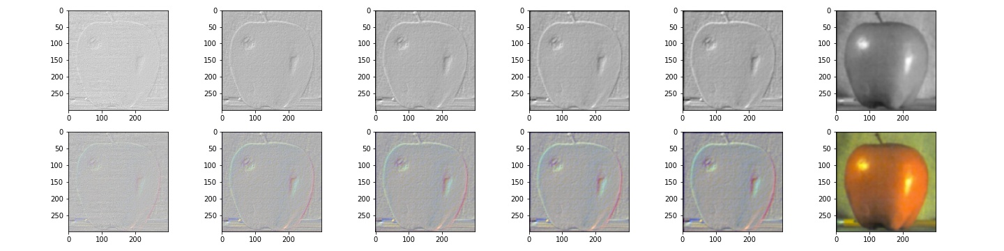
Apple Laplacian Stack
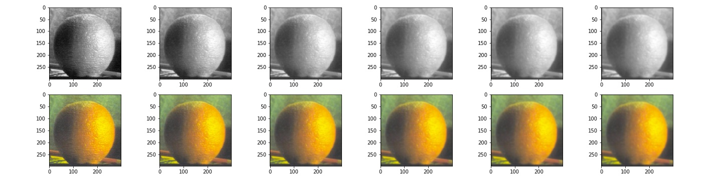
Orange Gaussian Stack
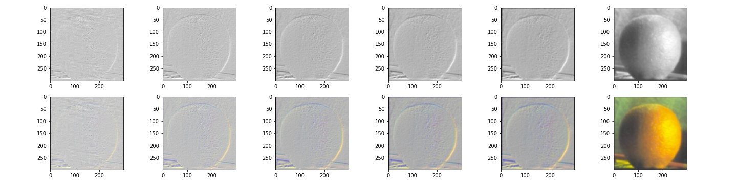
Orange Laplacian Stack
Half Apple Half Mask
Half Orange Half Mask
Half Orange Half Apple
We sum up the oraple Laplacian stacks and normalize the results to get the final oraple images below!
| Oraple Grey Image | Oraple Colored Image |
|---|---|
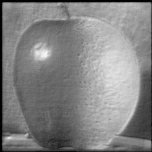 |
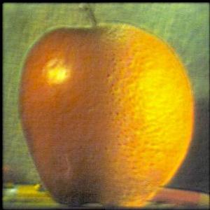 |
We definitely see that using color on images enhance the blending effect!

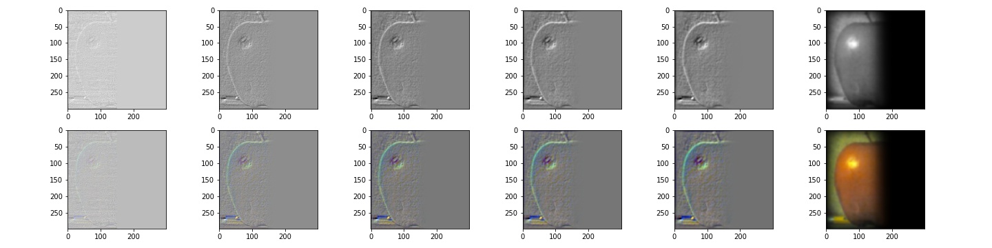
Seaoon Mask
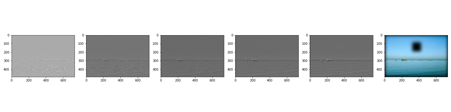
Sea Background
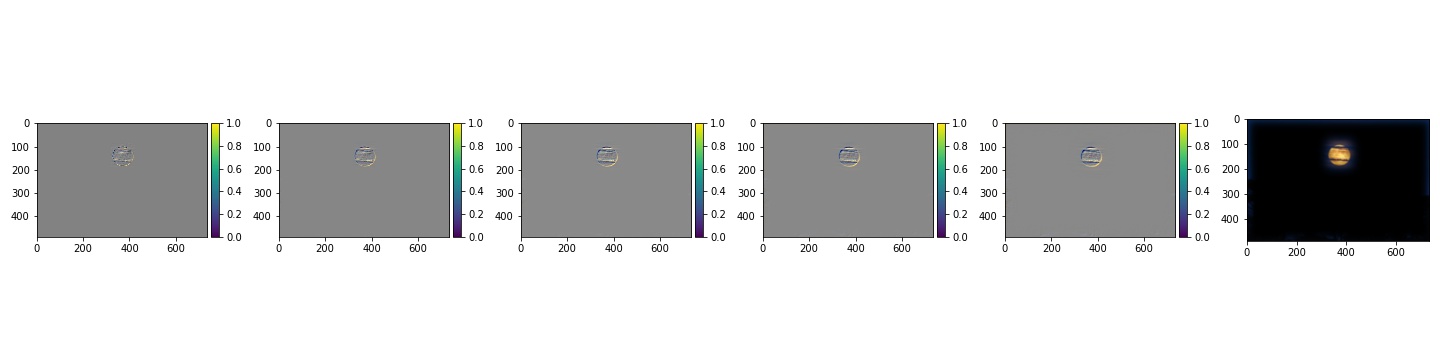
Only Full Moon
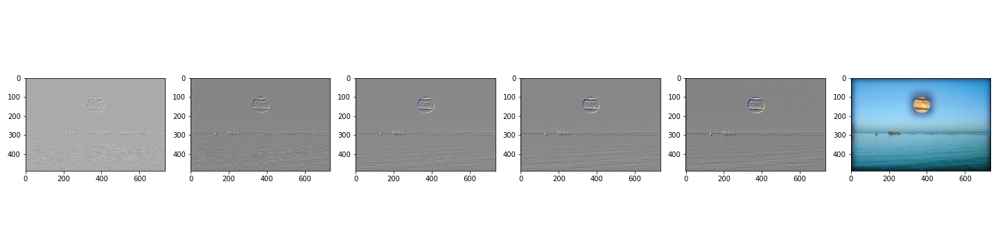
Sea Moon Blend Process
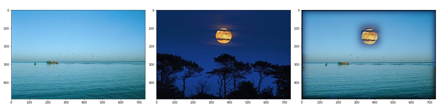
Seaoon

Mearth Mask
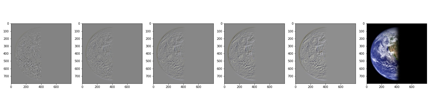
Half Earth
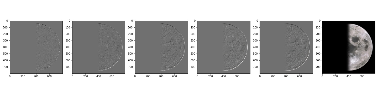
Half Moon
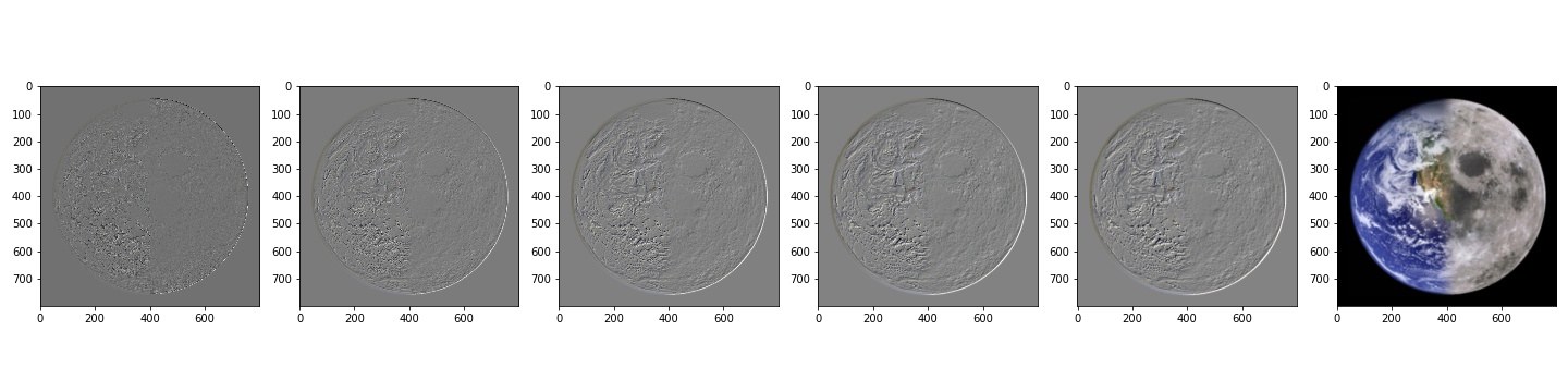
Moon Earth Blend Process
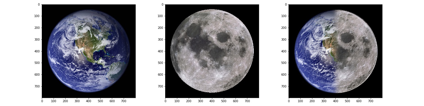
Mearth
The coolest thing I have learned from this assignment is that we can use Gaussian filter to help sharpen images. I find this very useful because I don't know any photoshop and now I can just use python to sharpen images!
The most important thing I have learned from this project is that normalizing/minmaxing images when visualizing really helps to bring out the features in the images.