Justin D. Norman Project 2: Fun with Filters & Frequencies!

Overview

The goal of Project 2 is to build and test intuition around the applications of image filtering and frequency modification.

1. Process & Approach

1.1

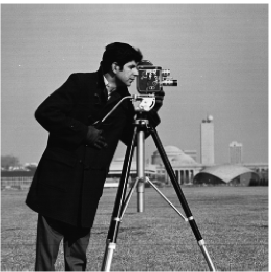
In this section, we were tasked with applying some simple techniques to the "Cameraman" image:

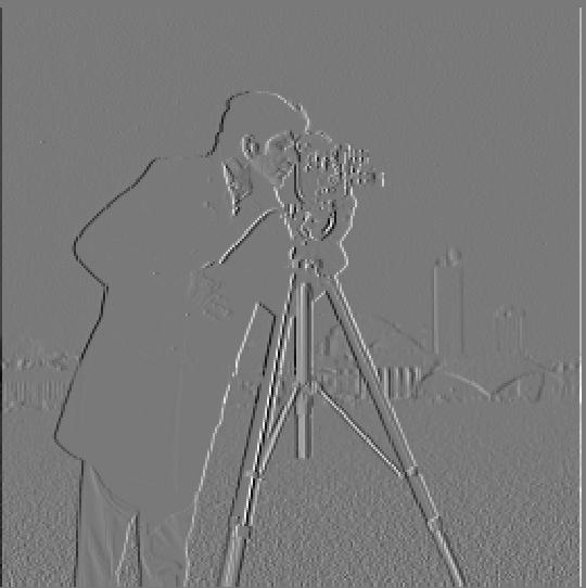
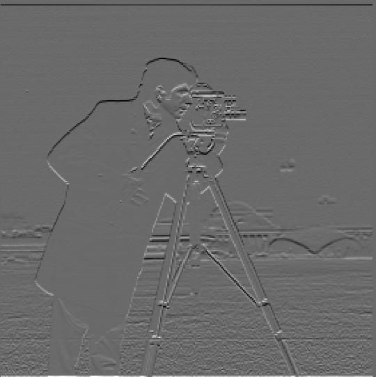
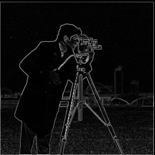
I explored using finite difference as an image filter by showing the partial derivatives with respect to x and y of famous image.

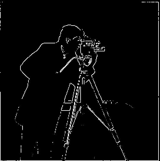
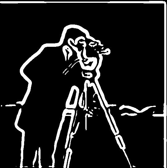
Next, the assignment called for computation and display of the gradient magnitude, which required me to convolve the D_x and D_y differentiation operators with the original image. Finally for this section, we were asked to binarize the gradient magnitude image to create an edge image, while also trying to suppress as much noise as possible. This required setting a threshold value of 0.39 and keeping the image array values between 0 and 1:

threshold, upper, lower = 0.39, 1, 0

1.2

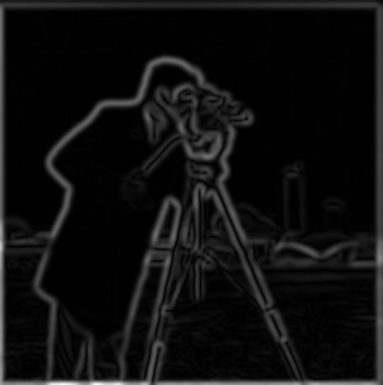
Because the binarized "edge" image was still quite noisy, the next step is to apply a smoothing technique--the Gaussian filter. We were tasked to create a blurred version of the original image, and then repeat the previous section, noticing the differences. The blurred version was achieved through convolving the original image with a Gaussian. In order to achieve this in python, it was necessary to first create a 1D Gaussian and then take an outer product with its transpose to get a 2D gaussian kernel.

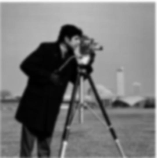
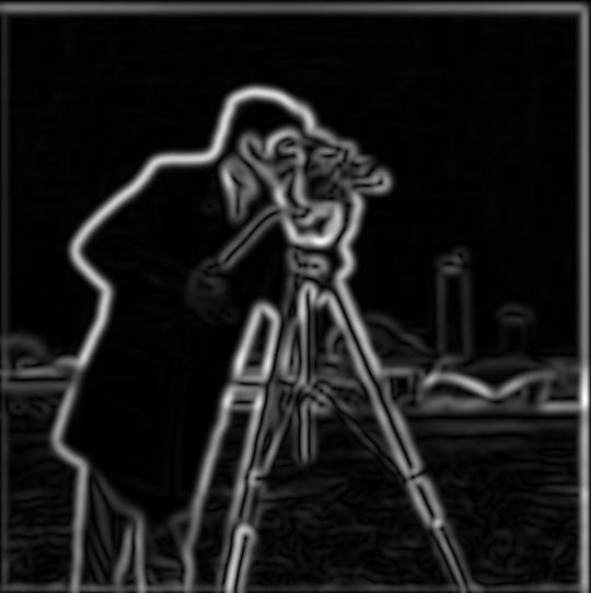
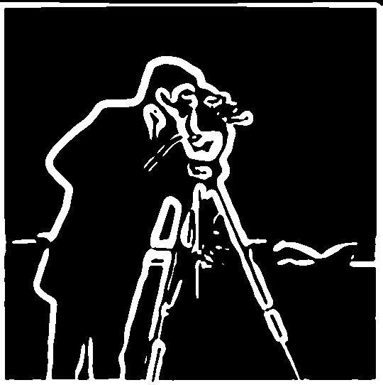
From the blurred image, repeating the gradient magnitude and binarizing processes, I noticed the following:

• Much more pronounced and thicker borders
• Higher edge detection of the bridge and less overall noise

The final part of this section asked us to verify that we could compute and display the same result using a derivative of Gaussian filters, which requires convolving the Gaussian just created above with the derivative images D_x and D_y, and then applying the following formula:

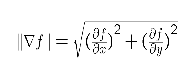
Below is the result:

Part 2: Fun with Frequencies!

Part 2.1 Image "Sharpening"

In this section we were tasked with deriving the unsharp masking technique: Subtracting the blurred version of an image from an original image to display only the highest frequencies of the image.

The more detailed technical procedure, executed in python, consisted of:

1. Splitting the image out into its (R,G,B) color channels
2. Constructing a Gaussian kernel
3. Obtaining the Blurred image from the convolution step
4. Executing the convolution
5. Reassembling the image's color properties

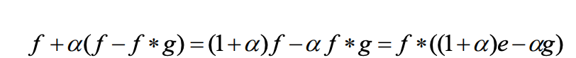
This can be done in a single convolution operation due to the definition of the unsharp mask filter as such:

For the example image, the steps are shown below:

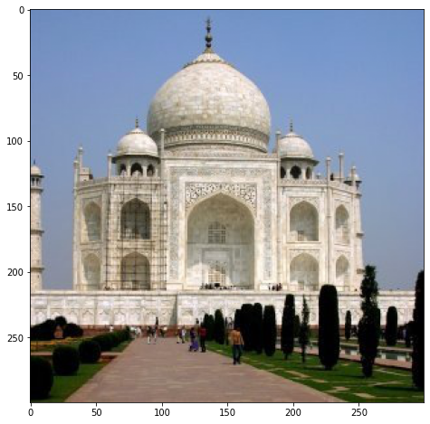
Left: Orignal, Right: "sharpened image

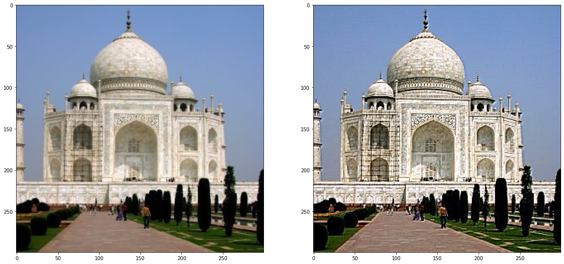
Next, we were asked to apply the methodology to our own images. I chose an owl image from the lecture slides. Below is the result of the image pipeline:

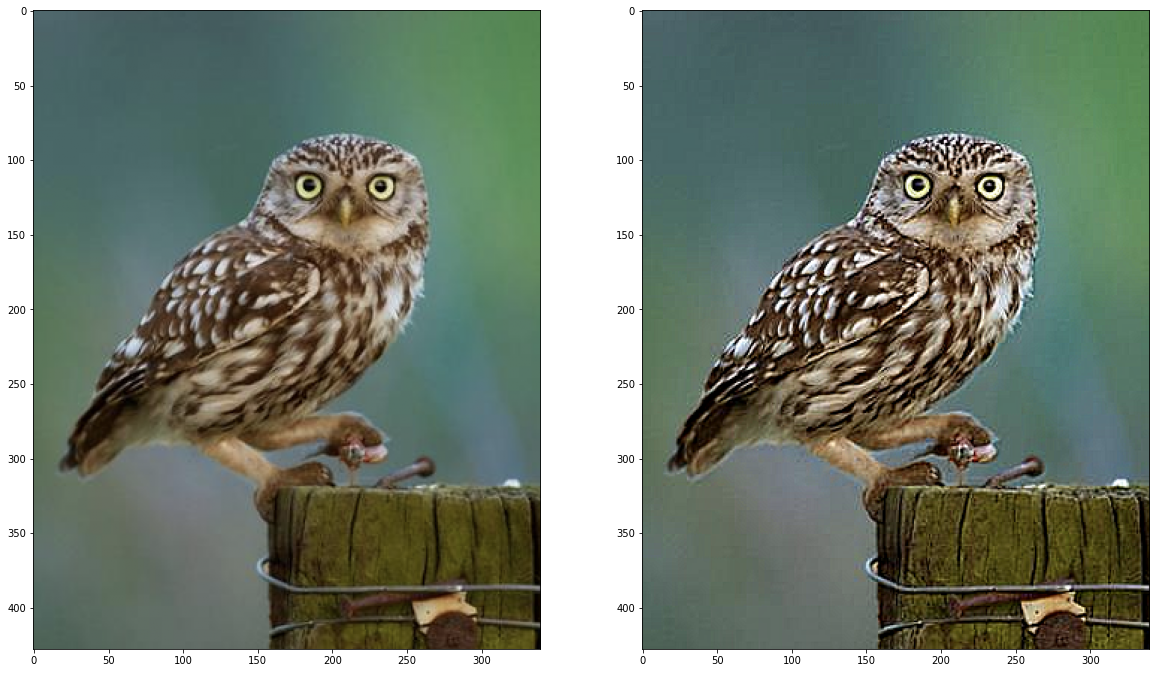
Some observations from both images include:

• The sharpening definitely brings out additional details of each image processed, but at a cost--there is clear distortion/loss of image signal in the "sharpened images"

• Choosing an alpha parameter for the single convolution step is non-trivial and was difficult to automate.

Part 2.2: Hybrid Images

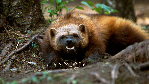
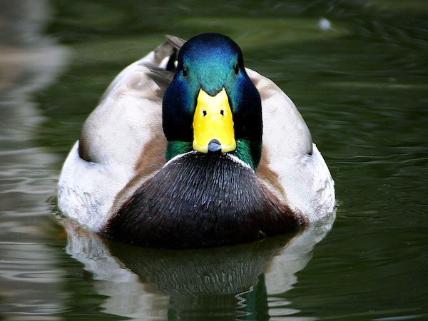
This section focused on the creation of hybrid images, which take advantage of the natural properties of human vision to prioritize high frequencies when available (when the eyes are close to the image) but farther away to process low-frequencies that are present. If a high-frequency portion of an image is blended with a low-frequency portion of another the effect of seeing different images at different distances or a "hybrid" is achieved.

The steps to achieve such an image in my solution are as follows:

1. Align the images
2. Make them both grayscale
3. Create a 2D Gaussian kernel for the low-frequency image
4. Apply the low-pass filter
5. Create a 2D Gaussian kernel for the high-frequency image
6. Define and apply the impulse kernel e (which is essentially an array with all 1s except at the center)
7. Average the two images

The input images are:

The results of the process on the given image, plus a couple of my own choosing are below:

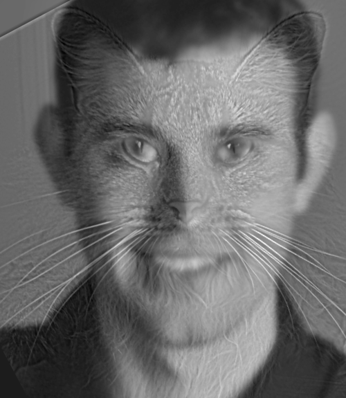
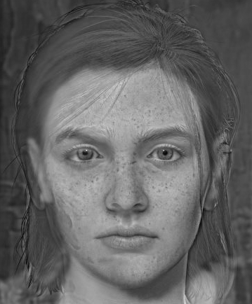
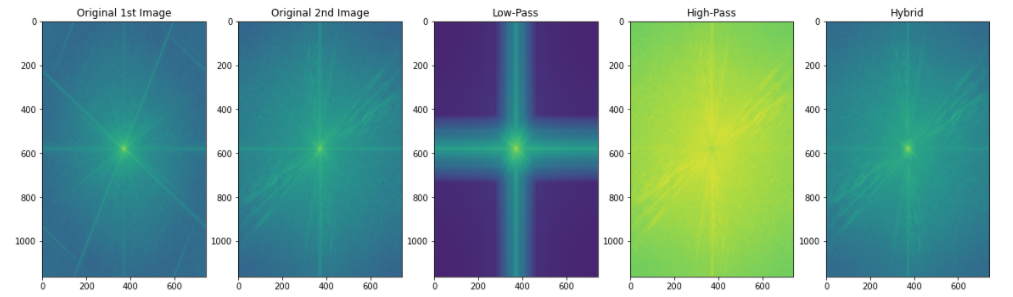
The log magnitudes of the fourier transform of the original first image, 2nd image, low-pass, high-pass and hybrid are below:

Part 2.3 Gaussian and Laplacian Stacks

This section consisted of two high-level steps:

1. Creating and visualizing the Gaussian and Laplacian stacks of two images and
2. Blending together the images with the help of the completed stacks, and exploring some interesting outcomes

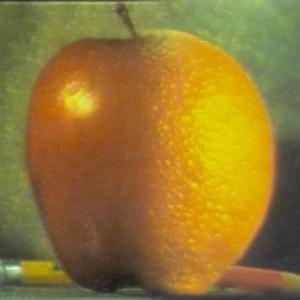
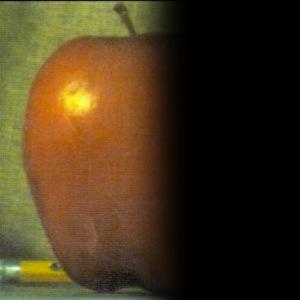
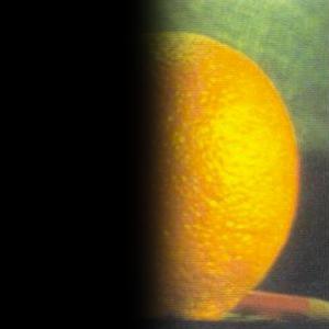
I first tackled this problem set using the given apple and orange images.

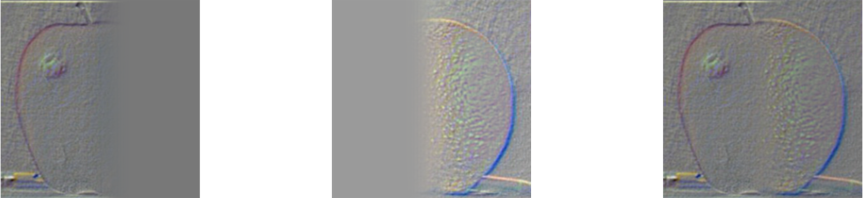
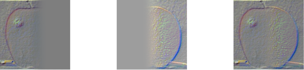
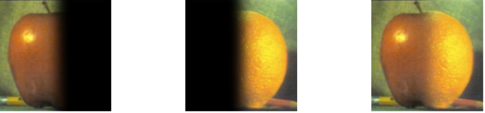
I then created the Gaussian and Laplacian stacks of both images, as you can see here:

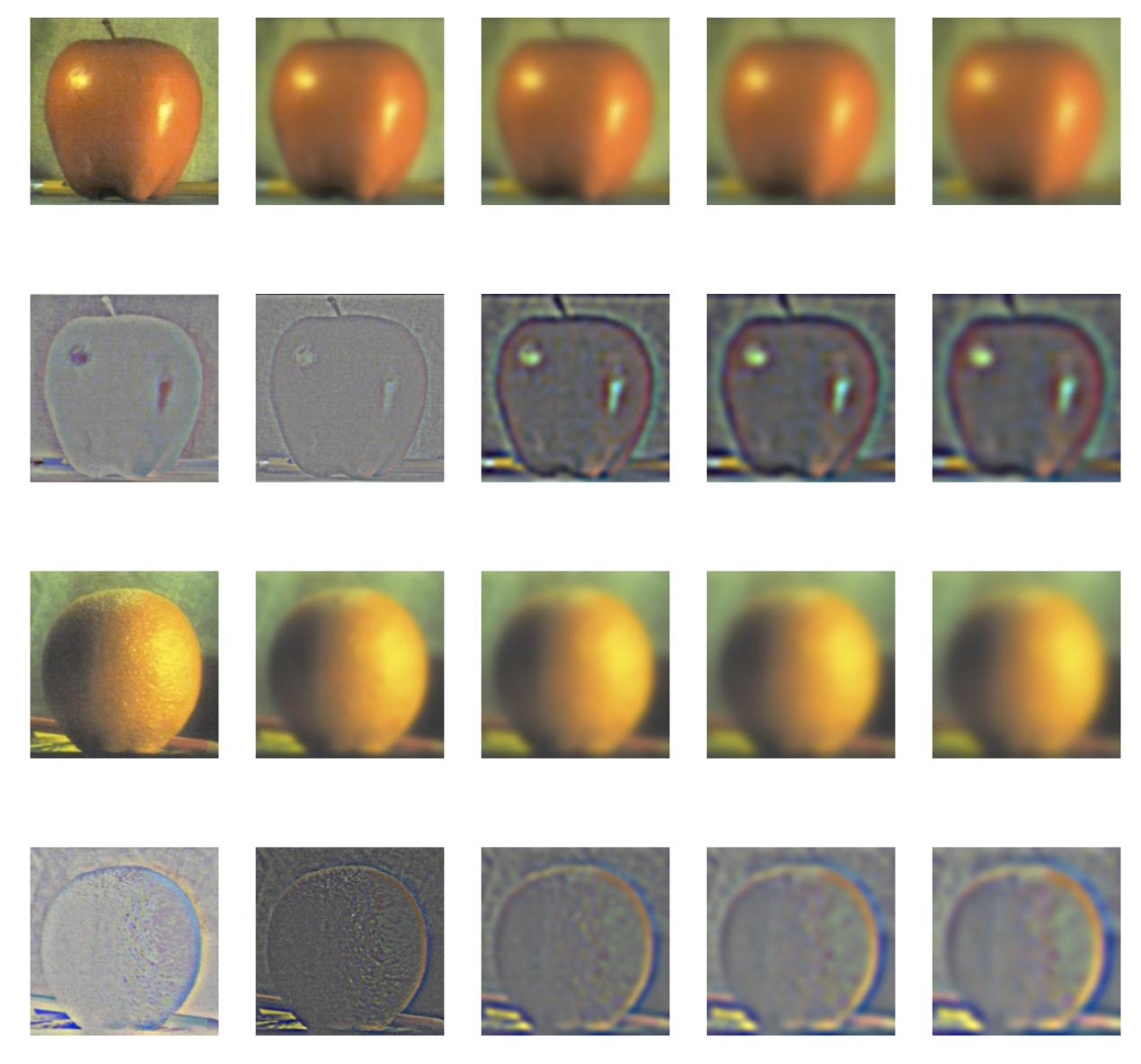
Using input from the next section, we can re-create the figure from the textbook:

Level 0

Level 2

Level 4

Combined

Part 2.4: Multiresolution Blending (a.k.a. the oraple!)

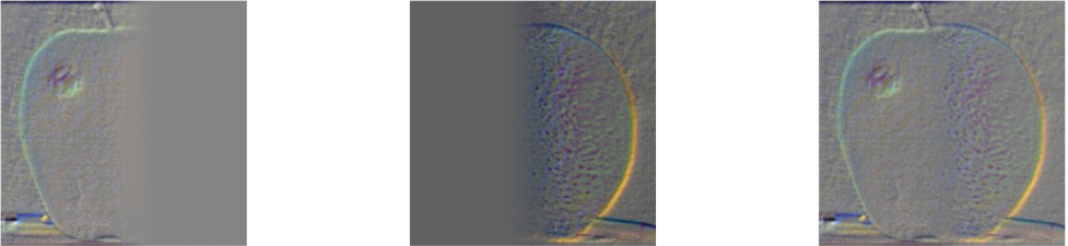
Using the same two source images from above, we proceed to blend the two pairs of images together. However, since we are running stacks not pyramids we need to implement the following process:

This is executed by:

1. Defining and applying a mask to both images, in this case just half of the image






2. Build Laplacian pyramids for both images

3. Build a Gaussian pyramid for the masked region

4. Create a combined pyramid, using the Gaussian mask as a weight

The result is a nice smooth blend of both fruits--and Oraple!: