Han Cui, SID: 3033631995
Email: louiscuihan2018@berkeley.edu
Section I: Fun with Filters
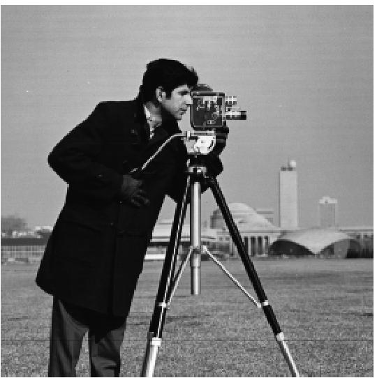
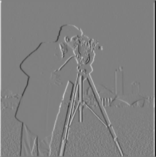
Part 1.1: Finite Difference Operator
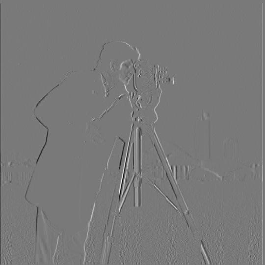
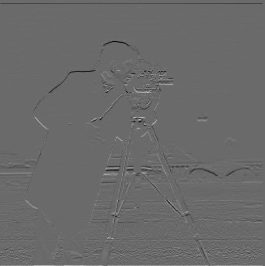
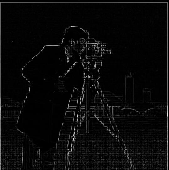
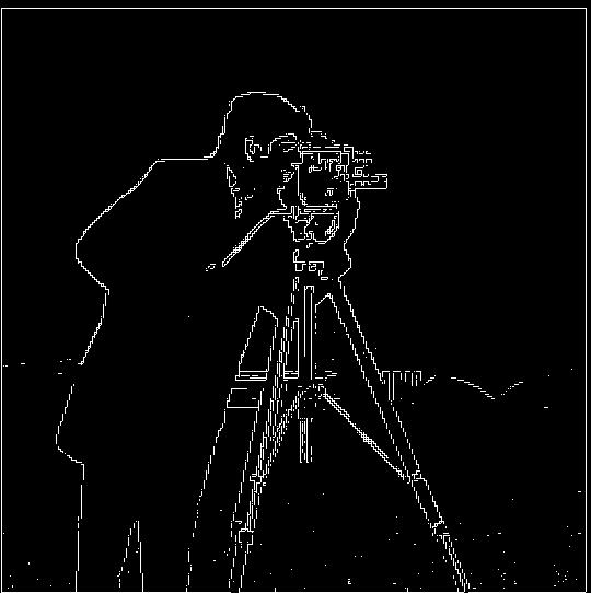
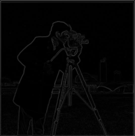
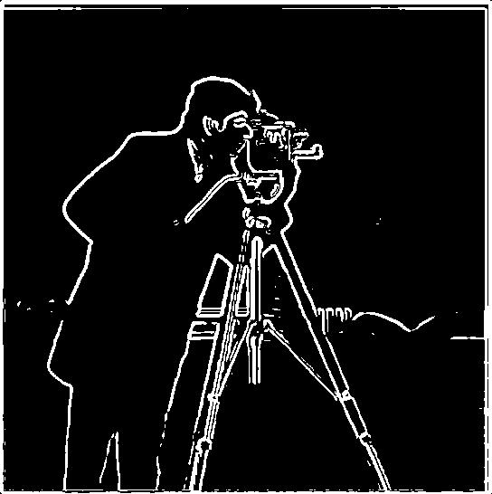
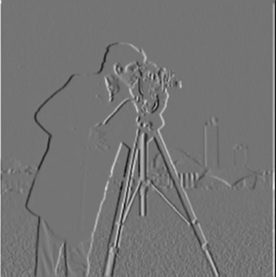
The way I compute the gradient magnitude image utilizes results from the convolution between the original image and Dx, and the convolution between the image and Dy. Given the formula $$ ||dI|| = \sqrt{\frac{dI}{dx} ^ 2 + \frac{dI}{dy}^ 2}$$ I use the Dx convolution and the Dy convolution as input to compute squares of each convolution result, and the square root of their sum. To generate the edge image, I binarize the gradient magnitude image with a threshold value of 0.26.
Part 1.2: Derivative of Gaussian (DoG) Filter
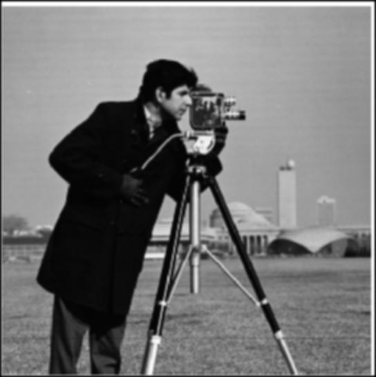
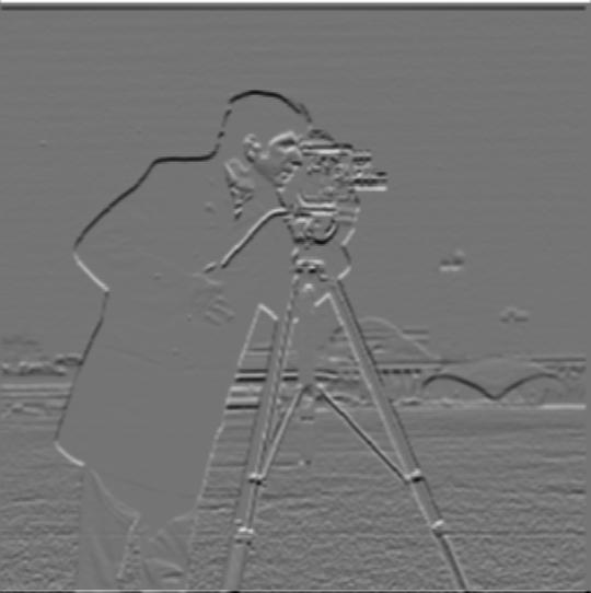
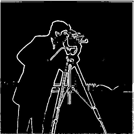
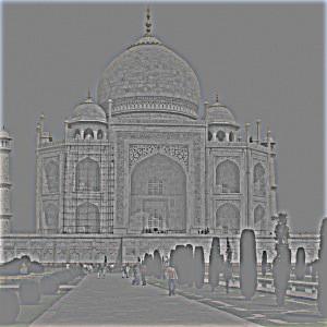
To get the results above, I use a Gaussian Filter of kernel size 5 and sigma 1.67 to blur the original image and run the same process from Part 1.1 on the blurred image. To get the results above, I use a Gaussian Filter of kernel size 5 and sigma 1.67 to blur the original image and run the same process from Part 1.1 on the blurred image. Compare to the results from Part 1.1, the images are darker, but the edges are thicker and thus more noticeable in the edge image. Since the results of this method are darker, I use a smaller threshold of 0.08 to get basic edges.
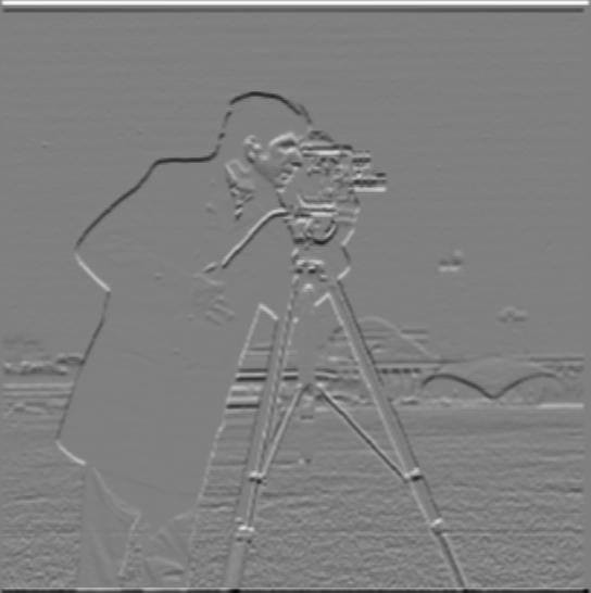
Another method to get strengthened edges is to use convolution to get the partial derivative Dx, Dy of the Gaussian filter, and then directly apply the DOG to the original image following a similar process. The results of this method, along with the visualizations of DOG, are shown below. Note these results are nearly the same, with the same parameters for the Gaussian filter and threshold value.

Section II: Fun with Frequencies
Part 2.1: Image "Sharpening"
The first method I use to "sharpen" images is the naive version: I first get the blurry version of the image by convolving it with the Gaussian Filter and then get the high-frequency image by subtracting the original image with the low frequency(blurry) image. Finally, I add the high-frequency data times a constant variable back to the original image to get the sharpened image. For all of the following experiments, I use kernel size 9 and sigma 3, and constant value 1.2. The formula is $$ I\_S = I + a(I - I\_B)$$
Another method for this image sharpening is to utilize an "unsharp mask filter". This method requires a Gaussian filter and a unit impulse filter to compute the unsharp mask filter and directly convolve it with the original image. The formula for this one is $$I\_S = I \circledast ((1+a)U- aG)$$ I show experiments with the unsharp mask filter method on the same image. Given the same parameters, two methods produce the same results.


Below are some more results. The unsharp mask filter truly brings a sense of sharper images.


Here is another set of experiments. I find a sharp image and blur it using the Gaussian filter. Then I try to use the unsharp mask filter to "re-sharpen" the blurred image. The process brings back some sense of sharp feeling, but it cannot bring the image back to its original since high-frequency information is lost and cannot be brought back by only the "sharpening" process.
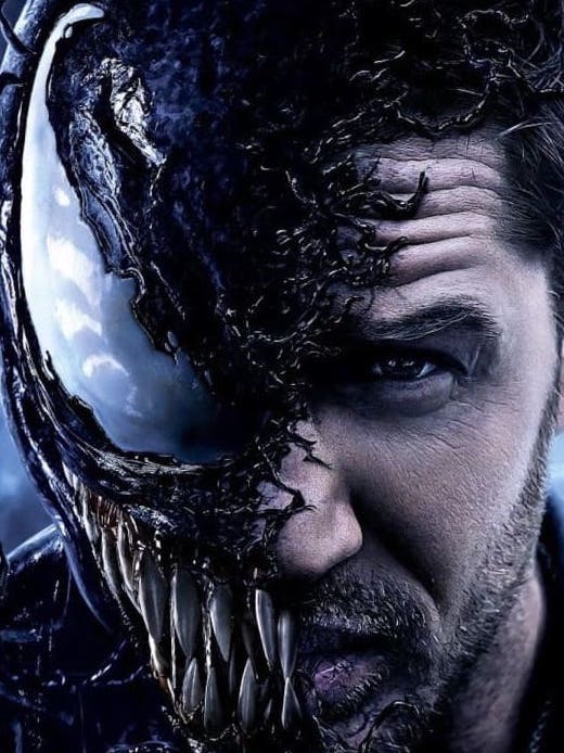
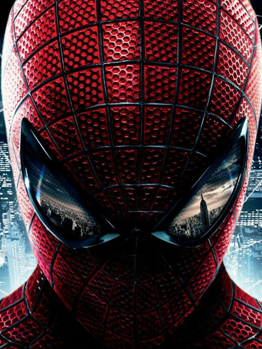
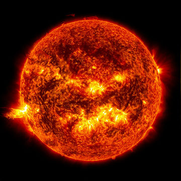
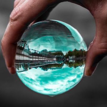
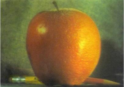
Part 2.2: Hybrid Images
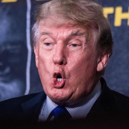
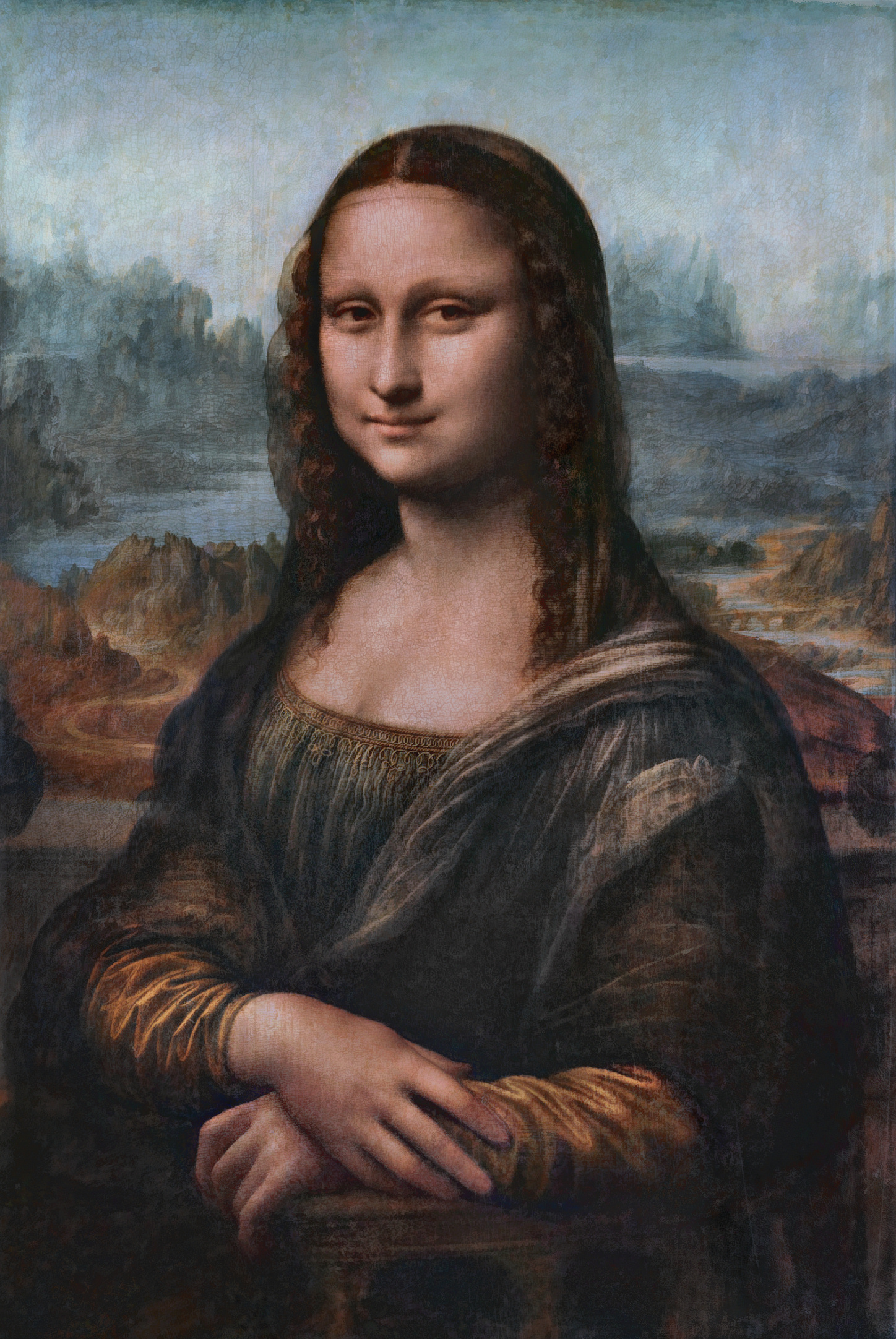
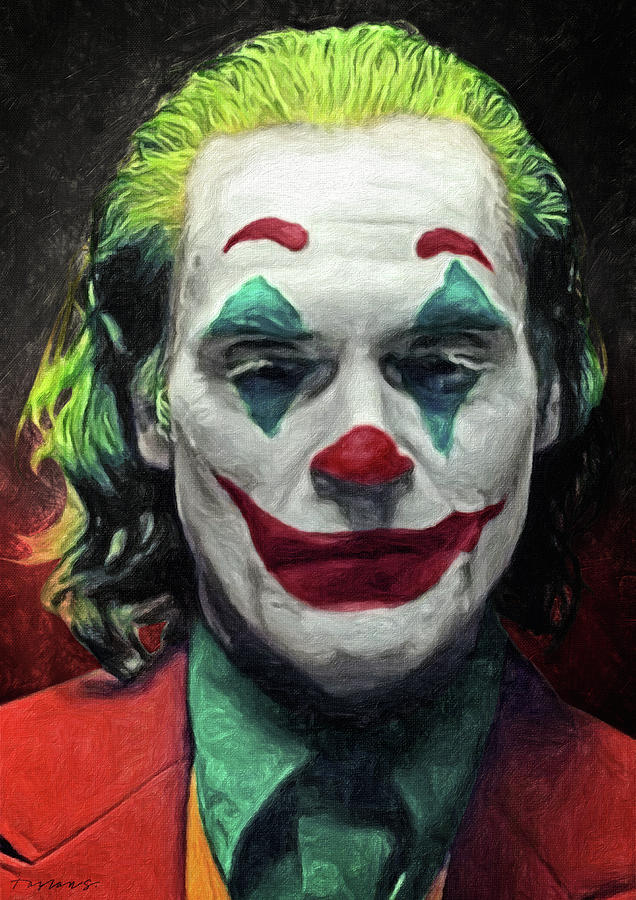
For the hybrid image, I use the method as the following: Here are some examples I select. After the two images are aligned, I extract a high-frequency image from one of the aligned images, and the low-frequency part from the other one. And I add up these two parts to form the resulting image. For all of the following results, I use the following parameters: kernel size for low freq image: 25, sigma for low freq image: 8.3; kernel size for high freq image: 25, sigma for high freq image: 20.

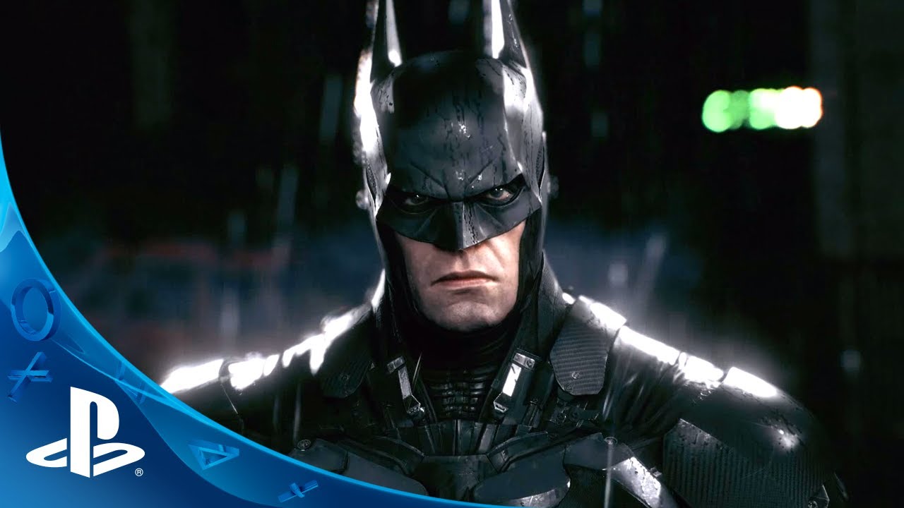
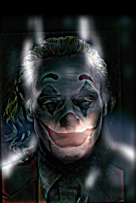

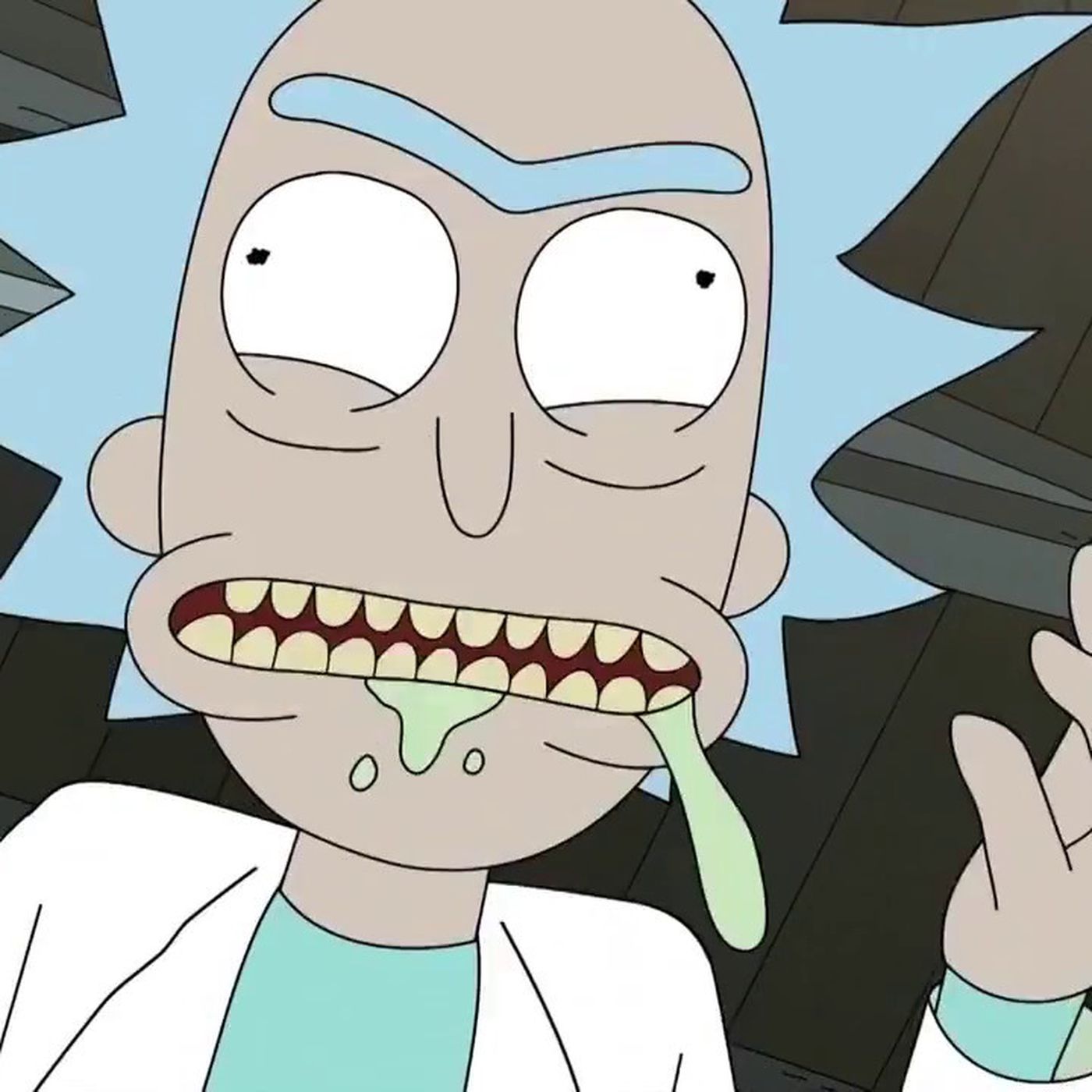
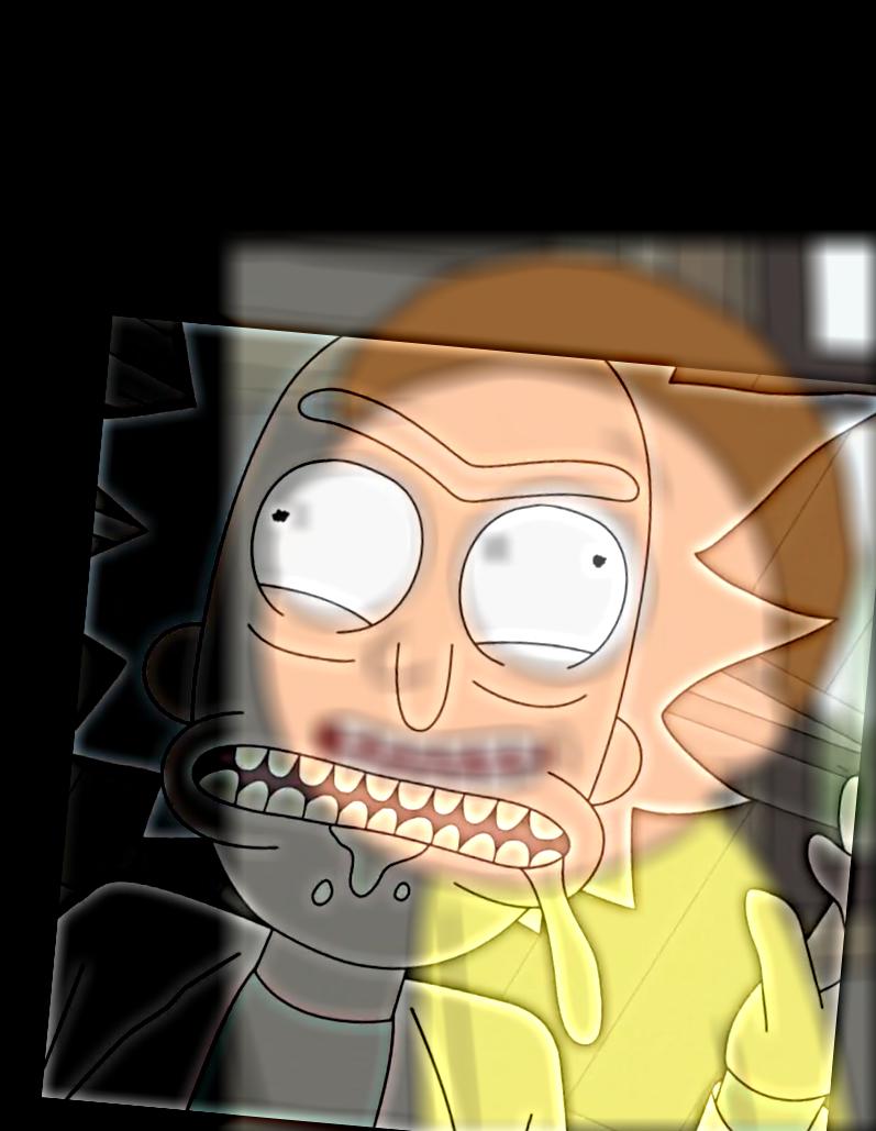
Here is one failure case: Rick and Morty don't hybrid well, because their pose and basic colors are so different from each other, which leads to both bad alignment and bad mixture after the hybrid, both contributing to the sub-optimal result.


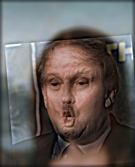
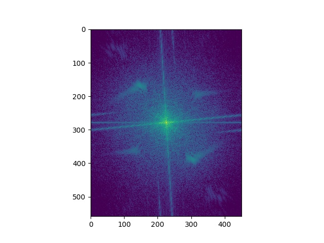
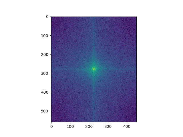
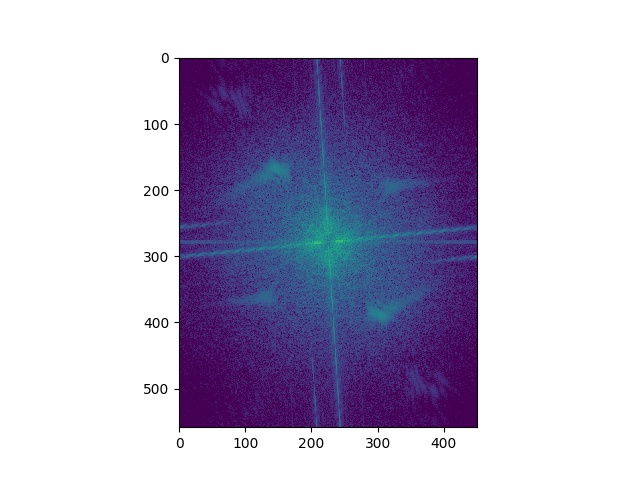
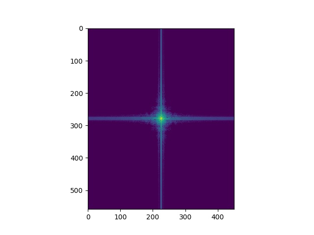
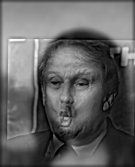
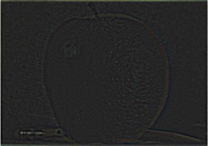
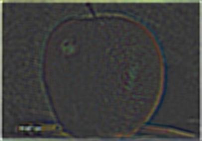
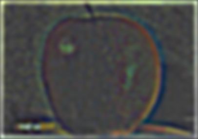
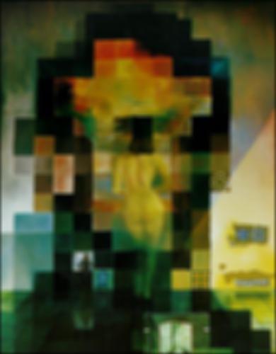
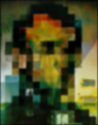
Here's the Fourier analysis of the "Trumalisa". As expected, the higher frequency has a missing central part in the frequency domain, and the low frequency only has central parts. And the sum of the two parts shows patterns of both images.
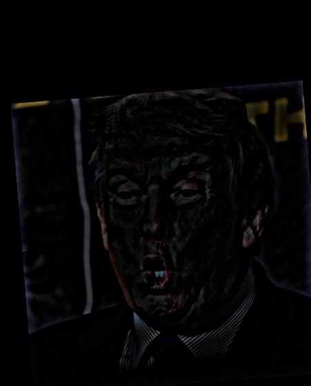
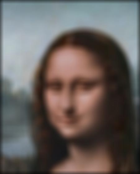

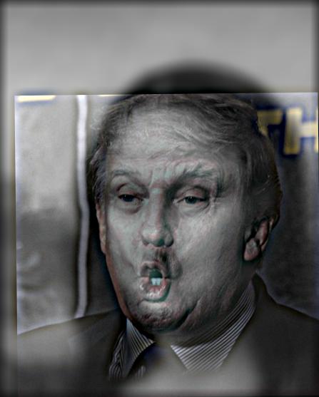
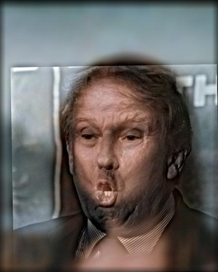
For the Bells & Whistles, I examined what could color play in the effects of hybrid images. In the ablation study, in the case where the high-frequency image is colored, the details look clear and vivid. For the cases where the high-frequency image is not colored, the hybrid images look odd in details of Trump's face edge, especially when Trump is gray while Monalisa is colored. However, this case study only covers the scenario where two alignments are nice and matching is good. For the case where the two objects look way too different, it is possible that both high and low-frequency images are gray can produce better hybrid images.


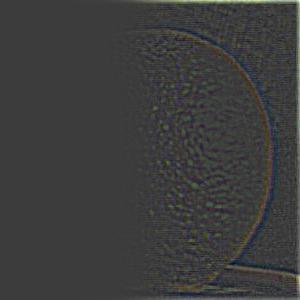
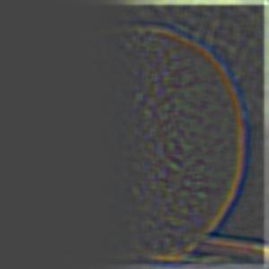
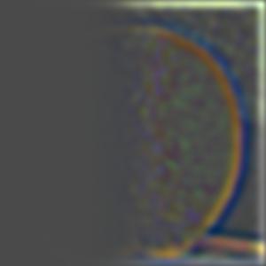
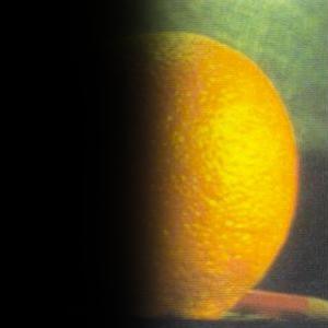
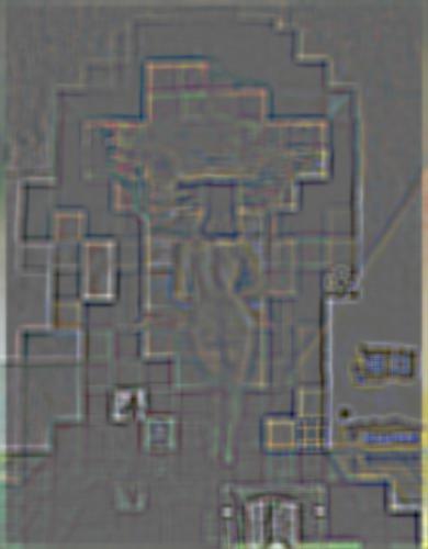
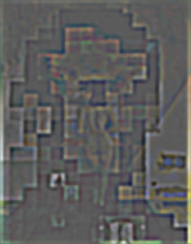
Part 2.3: Gaussian and Laplacian Stacks
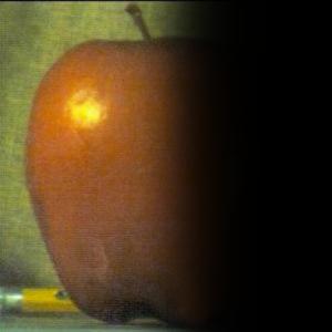
For this part, I first create Gaussian stacks of the original image by iteratively convoluting the image with a Gaussian filter, which thus contains low-frequency information with a different range. For the Laplacian stacks, I calculate the difference between the image and the Gaussian stack, or the difference between distinct layers of Gaussian stacks, which represent band-pass or high-pass filtered images. I use a Gaussian filter of kernel size 9 and sigma 4.5 for all experiments.
For these visualizations, each row represents the original image and different layers of the corresponding Laplacian stacks.

I also want to add some visualizations of Gaussian stacks and Laplacian stacks of the Lincoln image.


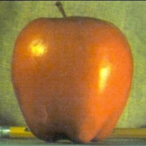
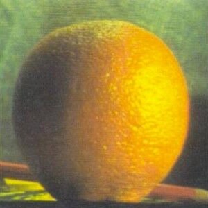
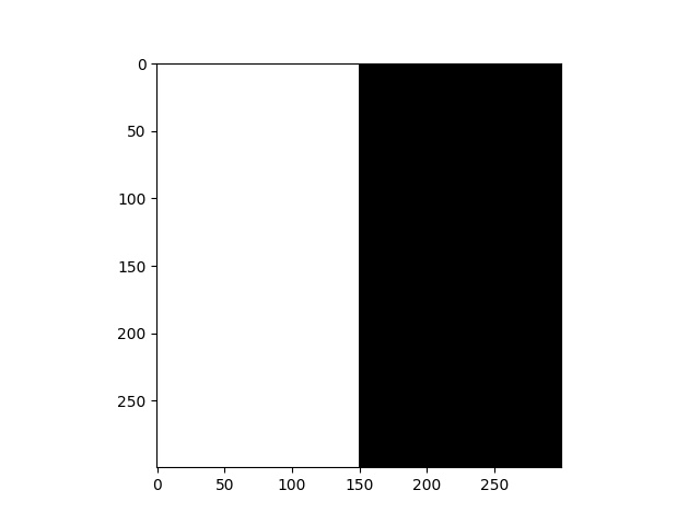
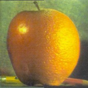
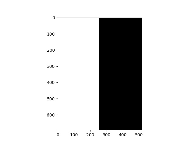
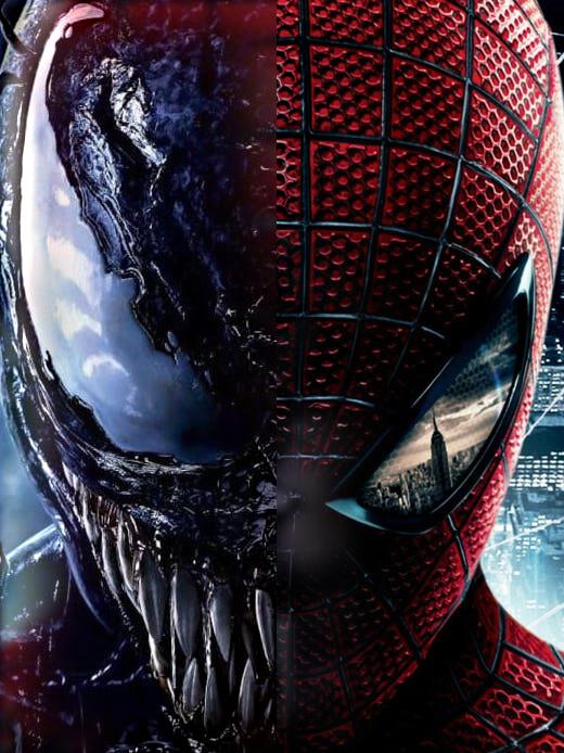
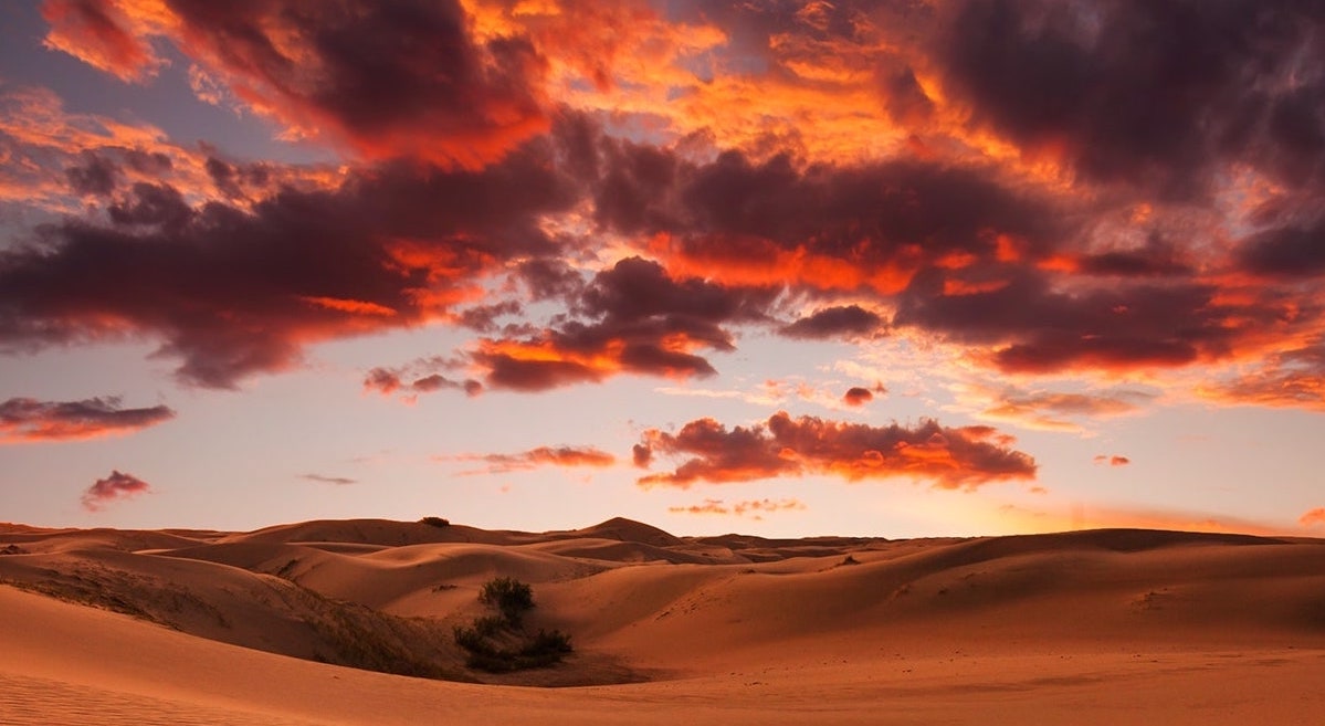
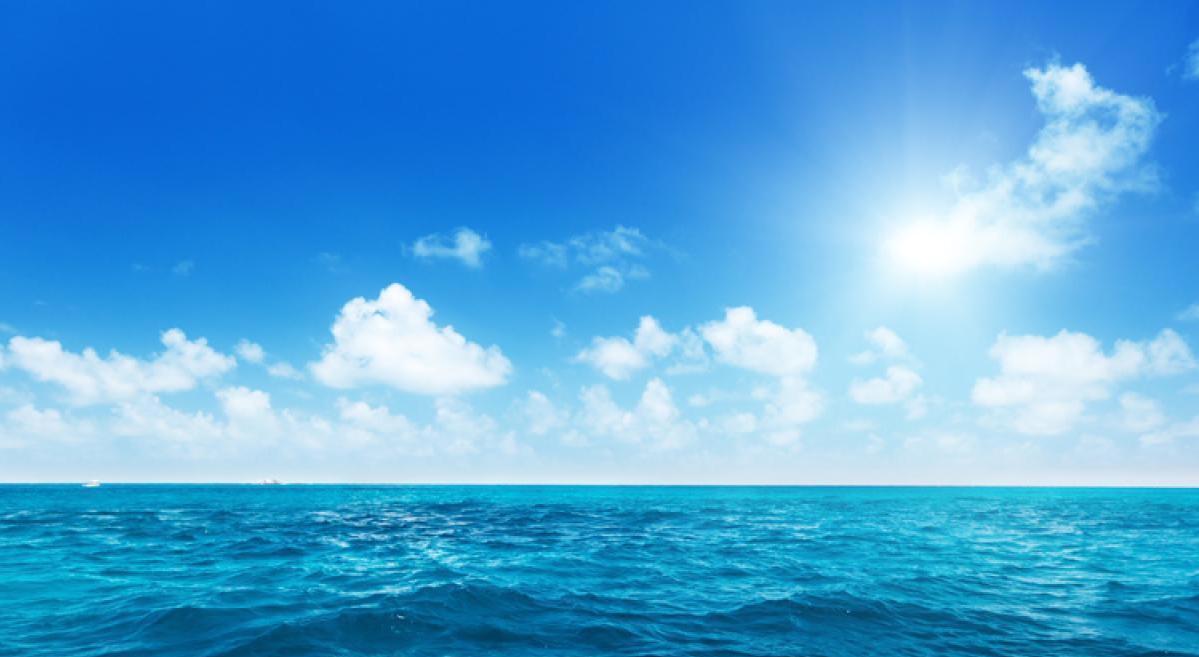
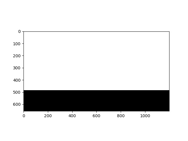
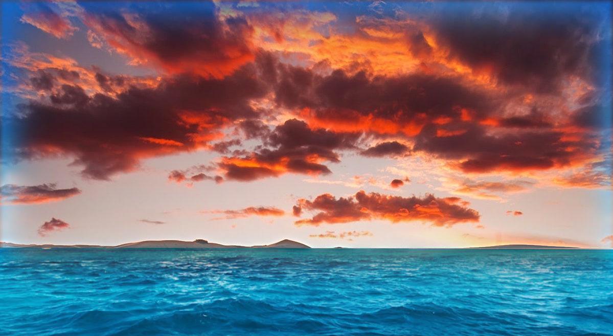
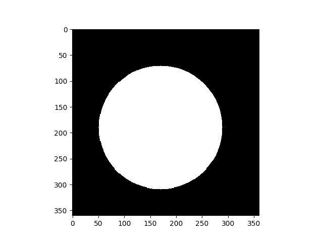
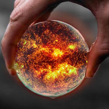
Part 2.4: Multiresolution Blending
For Multiresolution Blending, given two images Image_1 and Image_2, I first create a mask function of the same size. For the mask function, I first create the Gaussian stacks m; for two input images, I create corresponding Laplacian stacks l_1 and l_2. Given all of these stacks have the same number of layers, I add up each layer given the formula $$ result = result + m(i) * l\_1(i) + (1.0 - m(i)) * l\_2(i) $$
For the Bells & Whistles, I use color to enhance the blending, and for all following experiments, I use the following parameters: the number of layers 10; Gaussian stacks: kernel size 50, sigma 50; Laplacian stacks for both images: kernel size 17, sigma 5.