Lots of fun having in this project!

Part 1: Fun with Filters

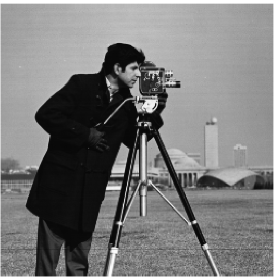
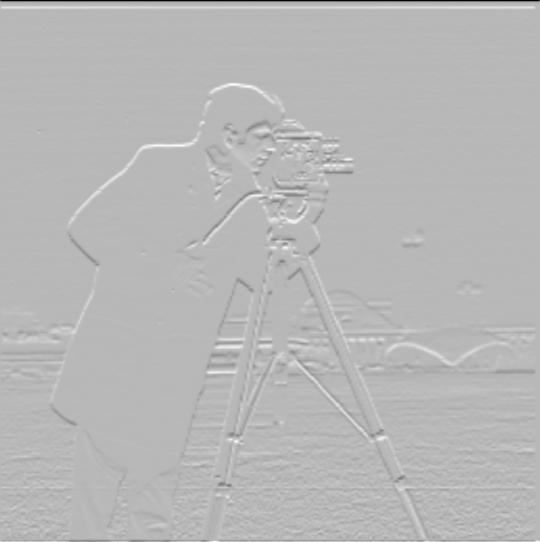
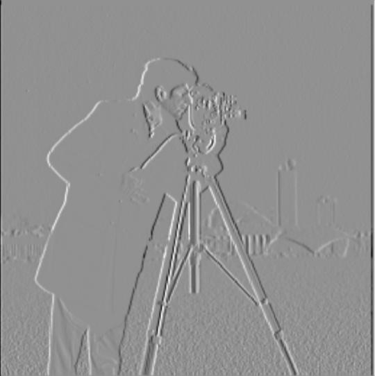
Part 1.1: Finite Difference Operator

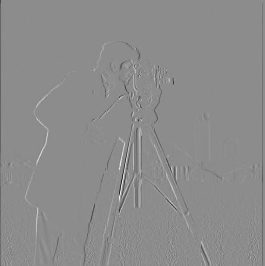
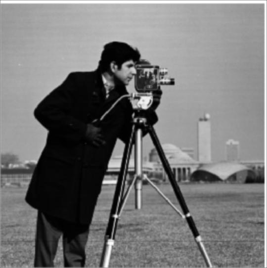
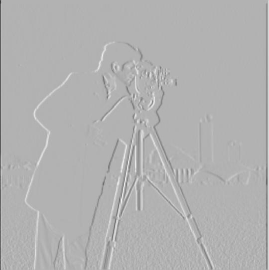
In order to compute the partial derivatives in x and y, we can convolve the image with the humble finite difference operators $\bold{D_x},\bold{D_y}$ such that

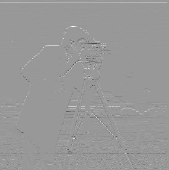
Next, we can combine these partial derivatives to compute the gradient magnitude image through the equation

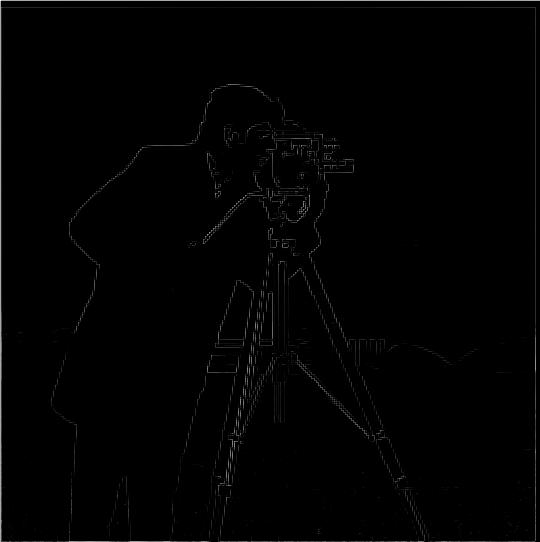
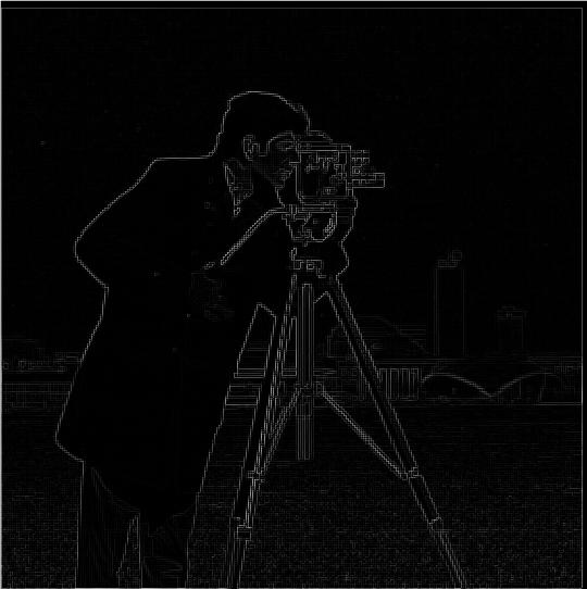
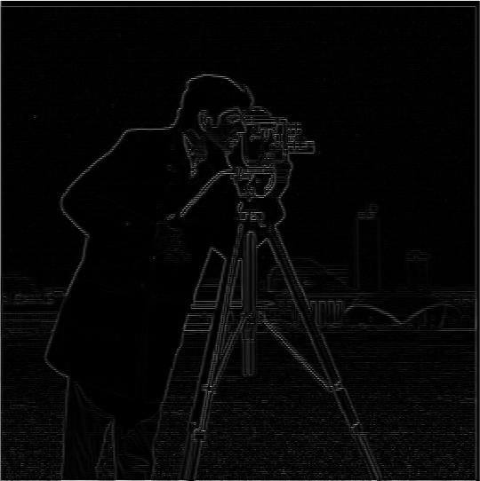
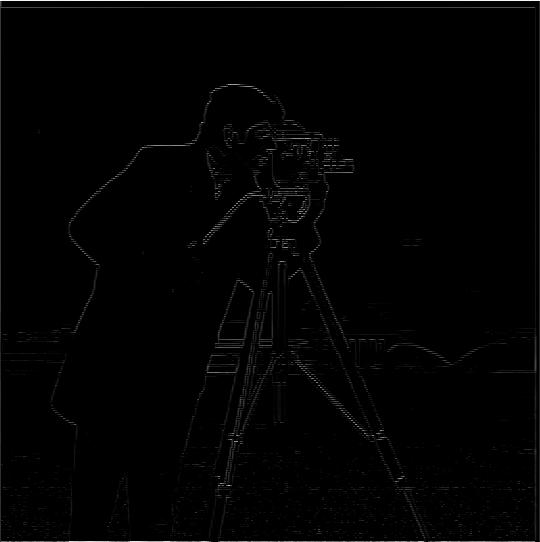
Finally, we can obtain an edge image by applying a minimum threshold to the gradient such that noisy edges are removed.

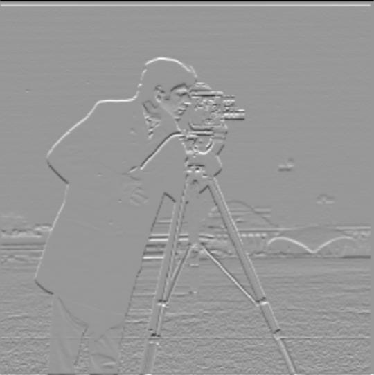
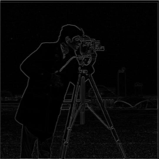
In this part, I calculate the partial derivatives, gradient magnitude image, and edge image through the methods described above.

Part 1.2: Derivative of Gaussian (DoG) Filter

In this subpart, I apply the method described in Part 1.1 on a blurred version of the original image to obtain a gradient and edge image with less noise using two methods:

Method 1: Blur Image first

This is the naive method where we first blur the image with a gaussian kernel, then apply the operation described in Part 1.1 to obtain the results:

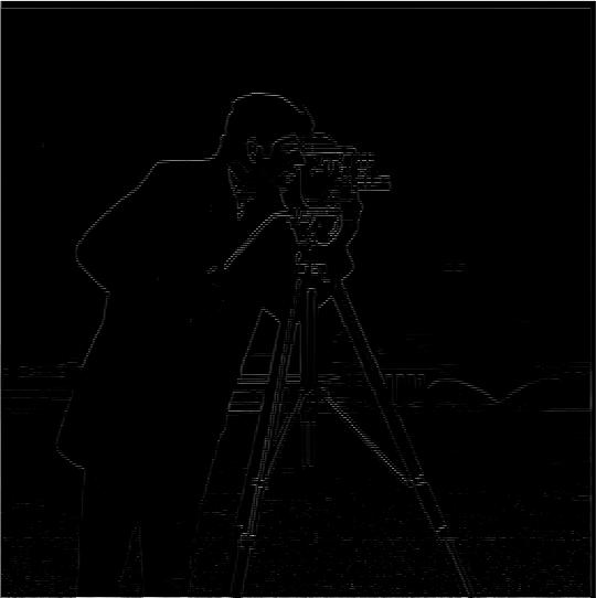
Comparing the edge_image of the original vs blurred images, we can see that the edge_image with blurring has less jagged edges and noise - best demonstrated by comparing the leftmost camera legs.

Method 2: Combine kernels first

In the second method, we first convolve the gaussian kernel with the finite difference operators, and then convolve the resulting kernel for each direction with the original image.

A visual inspection comparing the gradients of method 1 and method 2 show no noticeable differences which is expected.

Part 2: Fun with Frequencies

Part 2.1: Image "Sharpening"

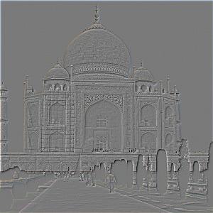
We know that blurring an image with a gaussian kernel will give us the low frequencies of the image. Now, if we subtract the blurred image from the original image, we can obtain an image of the high frequencies in the image. In this part, we will obtain the high frequencies of the image and increase them by a multiplier $\alpha$ to make images appear "sharper". These operations can be combined into a single convolution called the unsharp mask filter: $f*((1-\alpha)e-\alpha g)$, where $f$ is the image, $e$ is the unit impulse kernel(kernel of 0s with 1 in the center), $g$ is a gaussian kernel, and $\alpha$ is the sharpen amount.

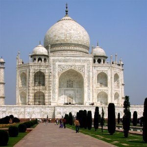
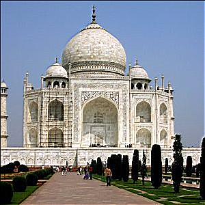
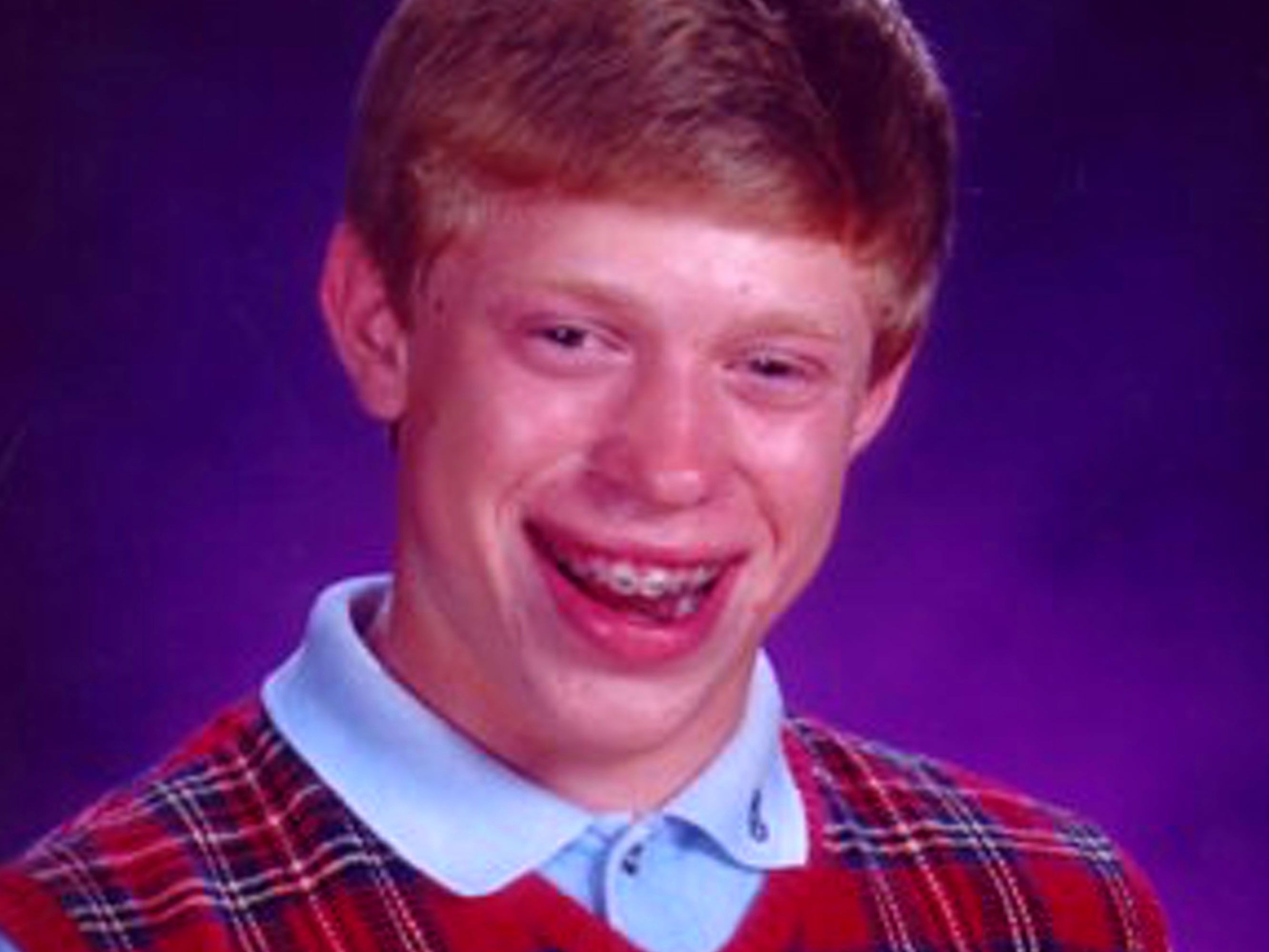
In this part, I apply the unsharp mask filter on some images. Here are some results:

Taj

Badluckbrian

Finally to evaluate this method of sharpening images, I have blurred an image of the campanile and will try to sharpen it again using the unsharp mask filter.

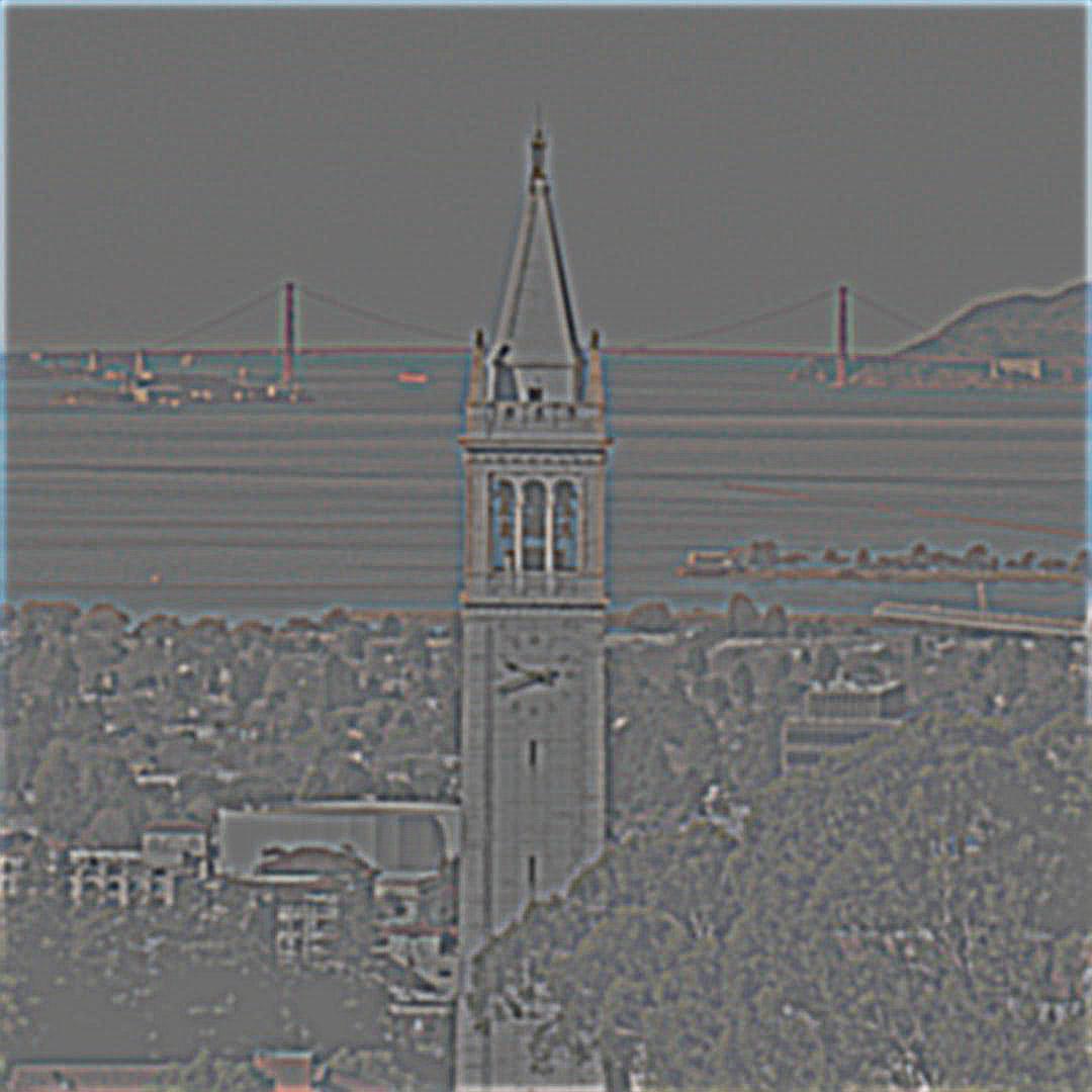
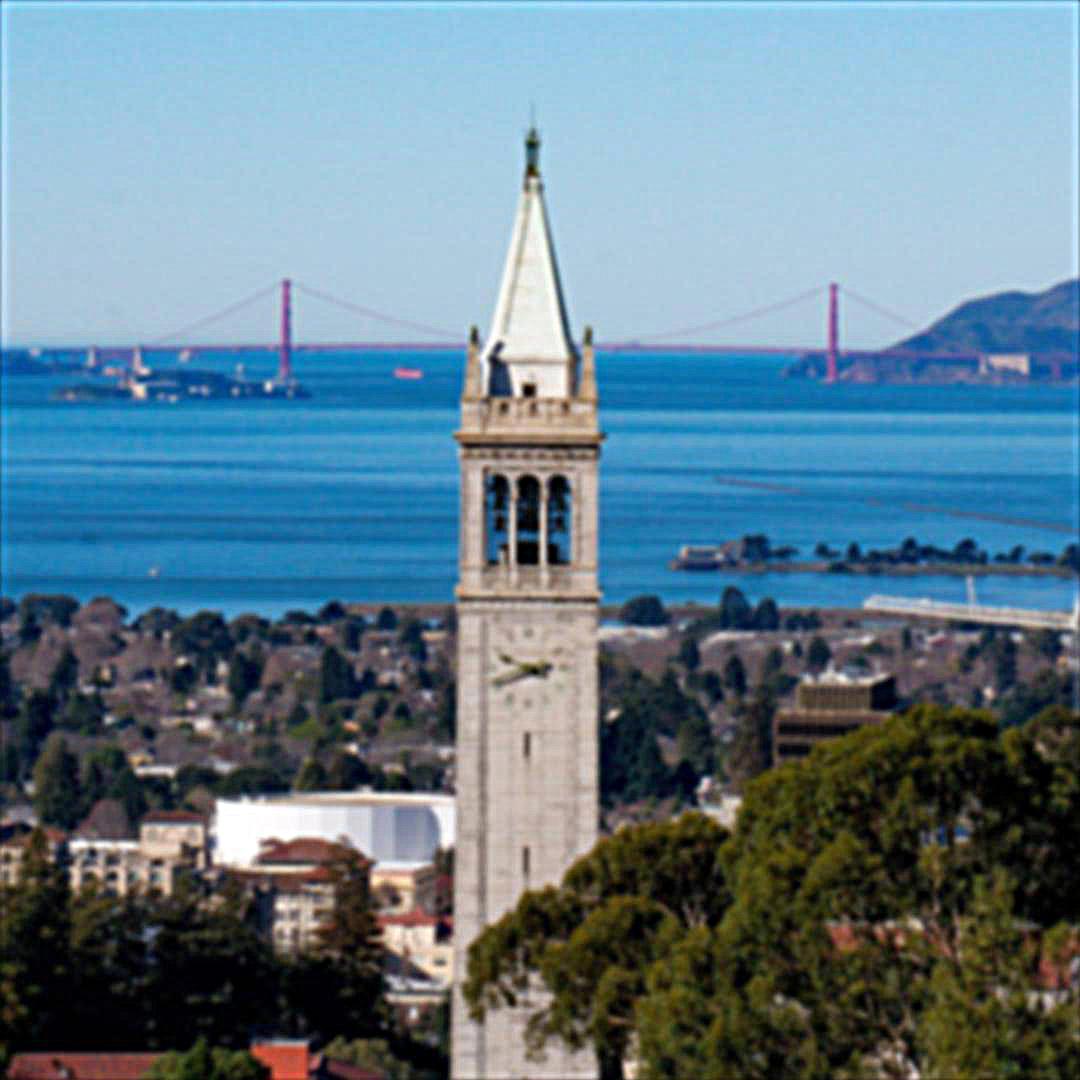
From the sharpened result of the blurred image, we can see that the result is now closer to the original campanile picture than the blurred version which is expected. The result isn't completely like the original however, as a visual comparison reveals that the sharpened result still appears a little blurry.

Part 2.2: Hybrid Images

Applying a gaussian kernel to blur an image acts like a low-pass filter on the image. Knowing this, we can also subtract an image by its blurred result to obtain an operation like a high-pass filter. In this section, I combine the low-frequencies of one image with the high-frequencies of another to form hybrid images that change in interpretation based on the viewer's distance. Specifically, these images will appear like one thing up close and something different from a distance. Here are some hybrid images I've generated:

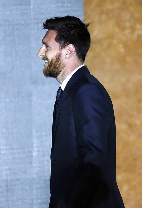
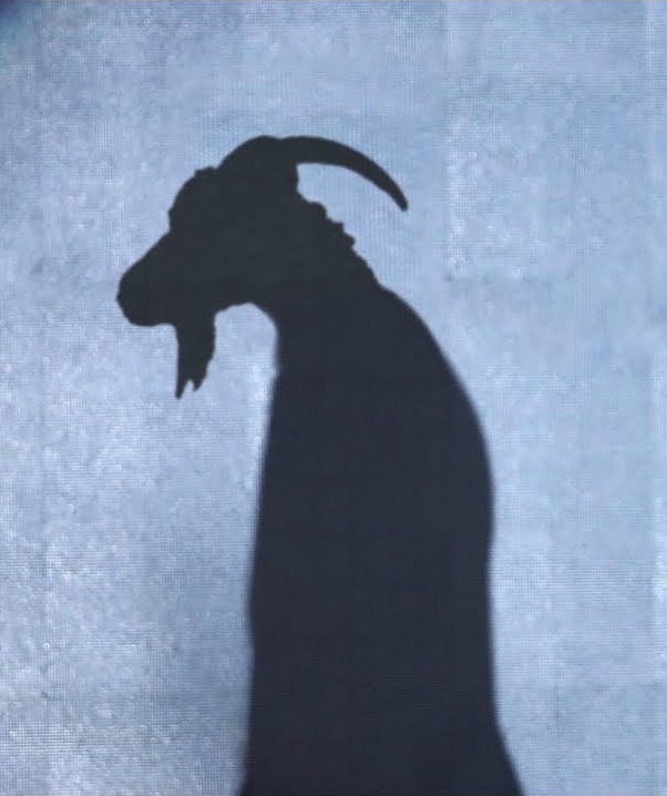
Messi Goat

Meme Galore

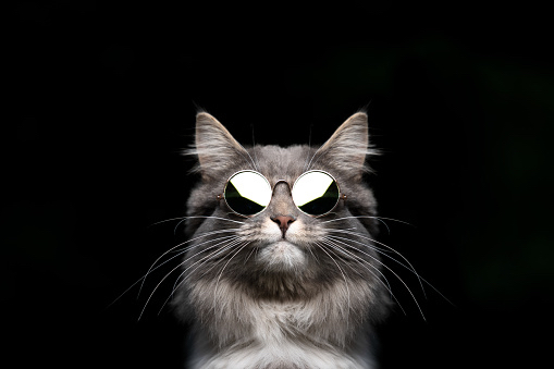
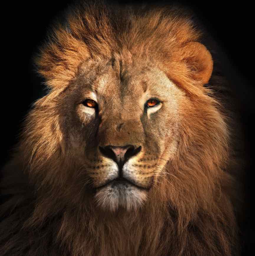
Coolcat Lion

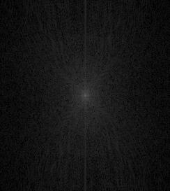
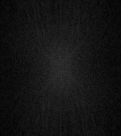
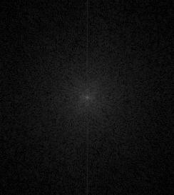
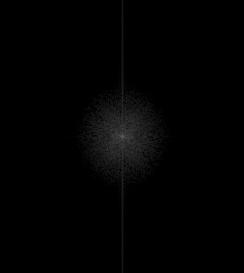
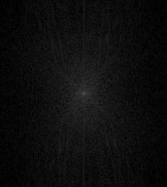
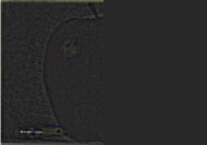
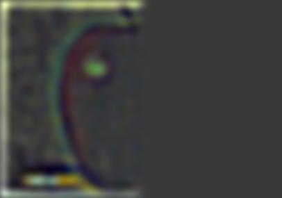
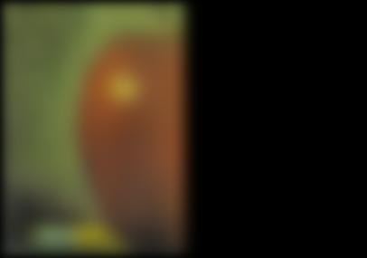
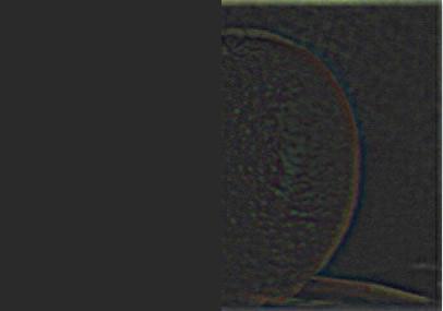
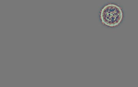
Fourier Transform Analysis for "Coolcat Lion"

We can gain some insight into the process of generating hybrid images using visualizations of the Fourier transforms. Here are the log magnitude plots of the Fourier transforms. We can see that the low frequencies are removed for the high pass transform and high frequencies are removed for the low pass transform.

Bells & Whistles for Part 2.2: I incorporated color in both the high-frequency and low-frequency components. I think overall the hybrid images look best when the low-frequency component has color and the high frequency one doesn't.

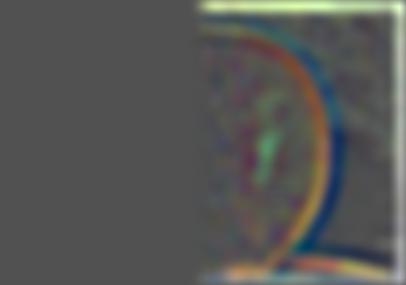
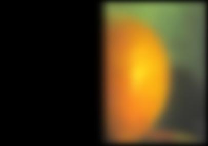
Part 2.3: Gaussian and Laplacian Stacks

A gaussian stack of height $n$ is a stack of images where every layer is obtained by applying a gaussian filter to the previous layer - with layer 0 being the original image. After constructing a gaussian stack, we can also construct a laplacian stack where $L_i$ is layer $i$ of the laplacian stack and $G_i$ is layer $i$ of the gaussian stack:

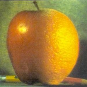
I generated gaussian and laplacian stacks with $n=5$ for the oraple and then applied a gaussian stack of masks to create two sets of masked gaussian and laplacian stacks.

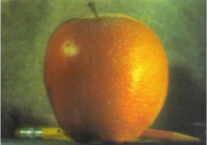
Oraple Gaussian Stacks

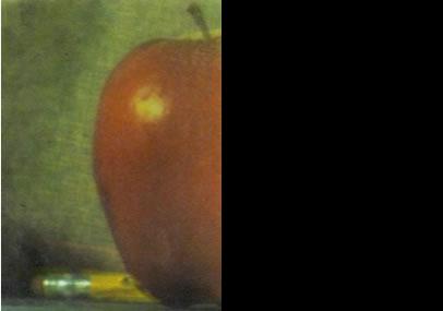
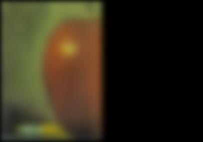
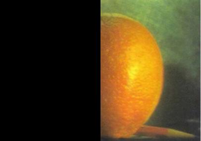
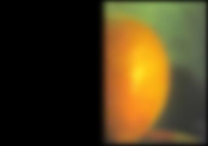
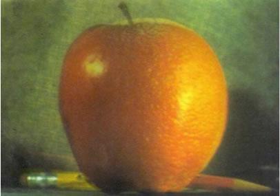
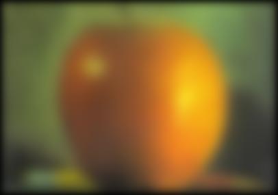
Oraple Laplacian Stacks

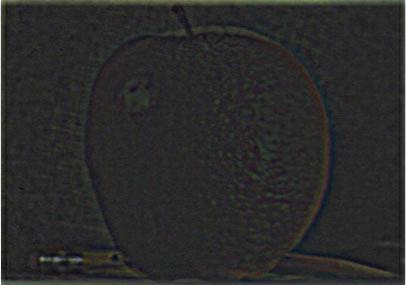
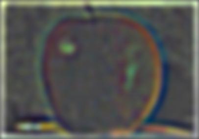
Part 2.4: Multiresolution Blending

In this section, I combine two laplacian stacks of different images with inverse masks to create hybrid images. I used photoshop to create the masks and align the images in order to create better looking results. Here are some example results:

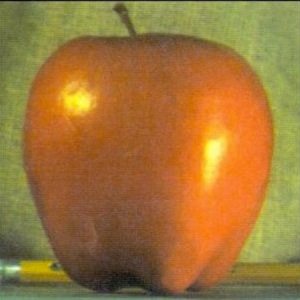
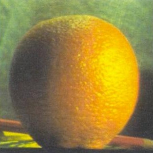
Apple + Orange = Oraple

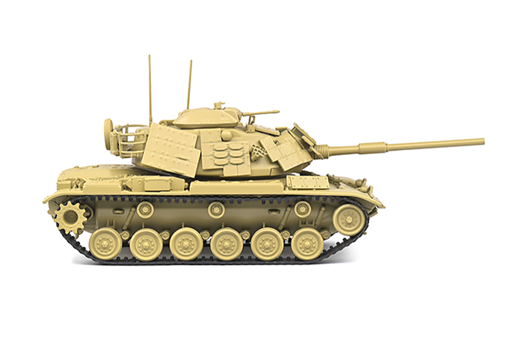
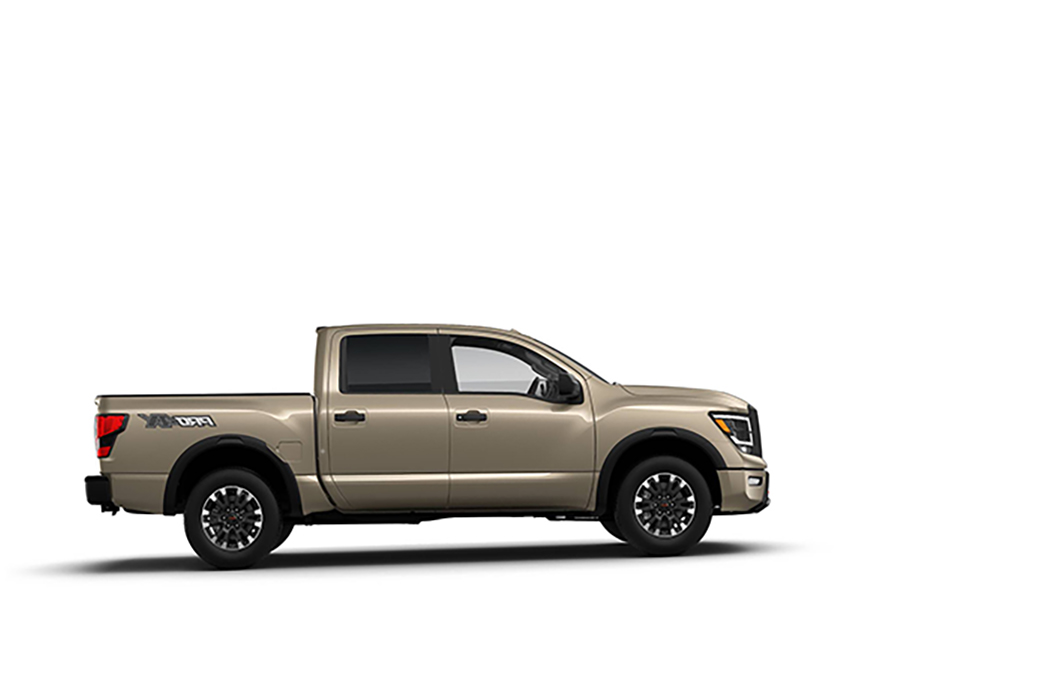
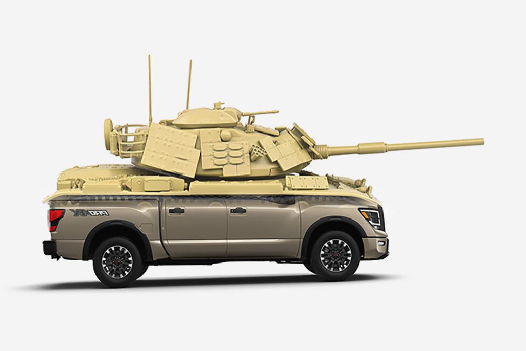
Tank + Truck = Trank?

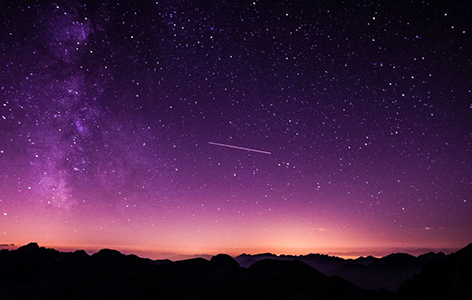
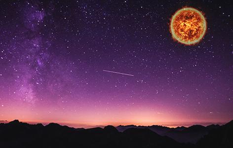
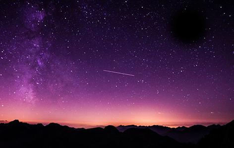
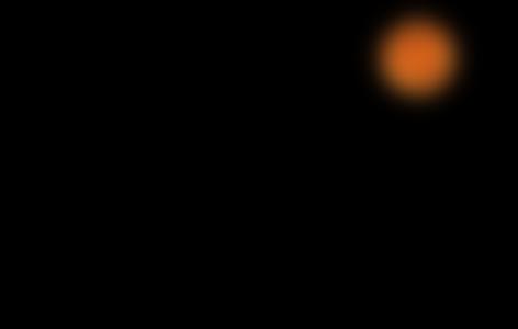
Night + Sun = A sunny night

Detailed Gaussian + Laplacian Stack for "A sunny night"

Here is a detailed breakdown of the gaussian and laplacian stacks that are used to create one of my example results.

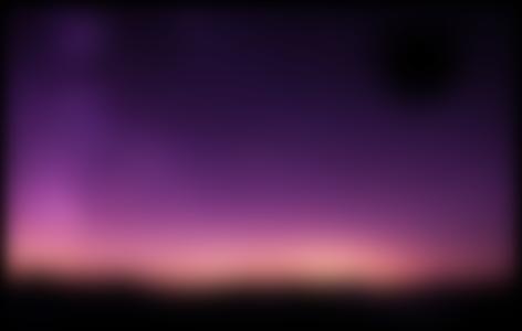
Bells & Whistles for Part 2.4: I also implemented the second part of the project with color. I think this turned out really well and looks especially good for the "A sunny night" example.

What I learned

How to do all of the methods described above as I didn't know how to do most of this stuff. More specifically, I think part 2 was especially interesting as it showed me how to think about images in terms of it's representation in the frequency domain.

I also learned about some weird interactions between using cv2.imread vs plt.imread and skio.imsave as cv2.imread ended up storing the channels in reverse order, so I had to perform an additional np.flip operation in my main.py file for part2.2(I spent 30 minutes debugging this).