CS 194-26 Project2

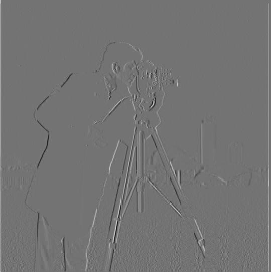
Part 1.1: Finite Difference Operator

Here are the resulting images:

Partial Derivative in x

Partial Derivative in y

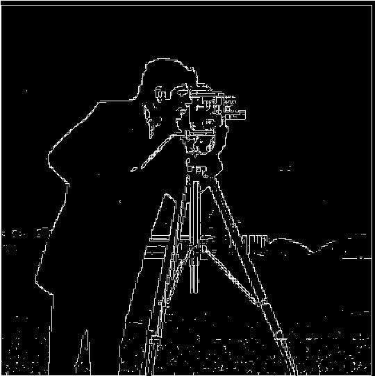
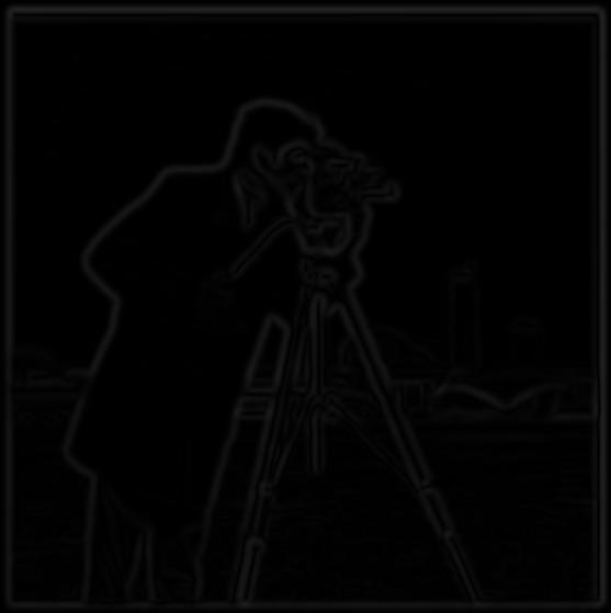
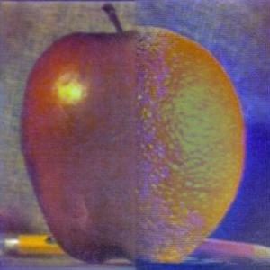
Computed gradient magnitude image:

gradient magnitude image

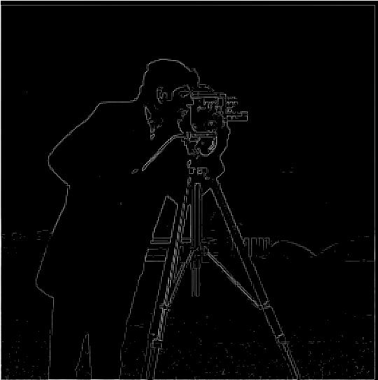
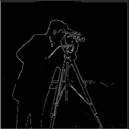
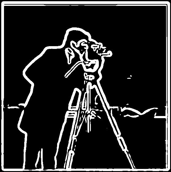
I used a threshold of 0.3, setting all values in the image that has value less than 0.3 to 0. I did some experiments around the threshold value, for example, here is the image output with a threshold of 0.2. The formula used to calculate the gradient magnitude is square root of ((partial derivative in x)^2 + (partial derivative in y)^2)

edge image with threshold=0.3

edge image with threshold=0.2

we can see that there are still a moderate amount of noise in the background in the very bottom of the image. On the other hand, the amount of noise is reduced with threshold 0.3

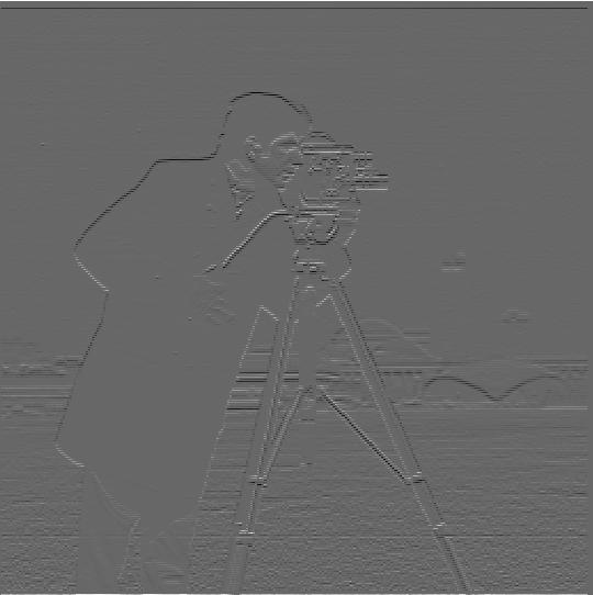
Part 1.2: Derivative of Gaussian Filter

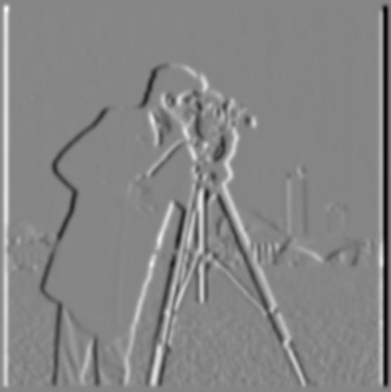
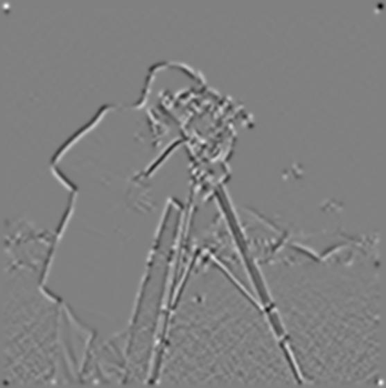
1.2.1 Blur the image first, then apply partial derivative

Gaussian blurred cameraman image

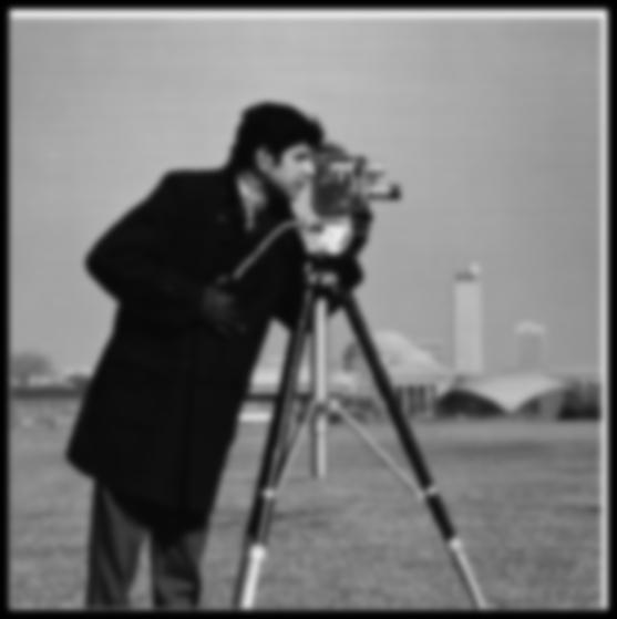
The image differs from the one generated from Part 1.1 in the way that the edges are more visible. That is because blurring the image suppresses the noises in the image.

Gaussian convolved X	Gaussian convolved Y
Calculated gradient magnitude	Binarized gradient magnitude (edge) image using a cutoff frequency of 0.03
Original image convolved with X and Y

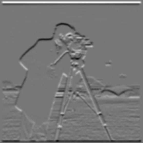
1.2.2 Convolve Gaussian with partial derivatives and filter the image

Final resulting image

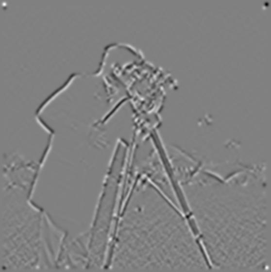The image is the same as the output image in 1.2.2. Because convolving is a communtative operation, so

1. convolve image with partial_x

2. convolve resulting image from step1 with partial_y

3. apply gaussian filter to resulting image in part 2

is the same as

1. convolve gaussian filter with partial_x

2. convolve result from step 1 with partial_y

3. filter the image with the filter calculated in step 2

Part 2.1 Image "Sharpening"

For this part, I show the result of sharpening of the taj image, plus two of my favorite images I took in Yosemite National Park.

The original taj image	Sharpened taj image
The original Yosemite image	Sharpened Yosemite image
The original Yosemite-camera image	Sharpened Yosemite-camera image

We can see that after sharpening, the edges of the shapes in the image is more visible.

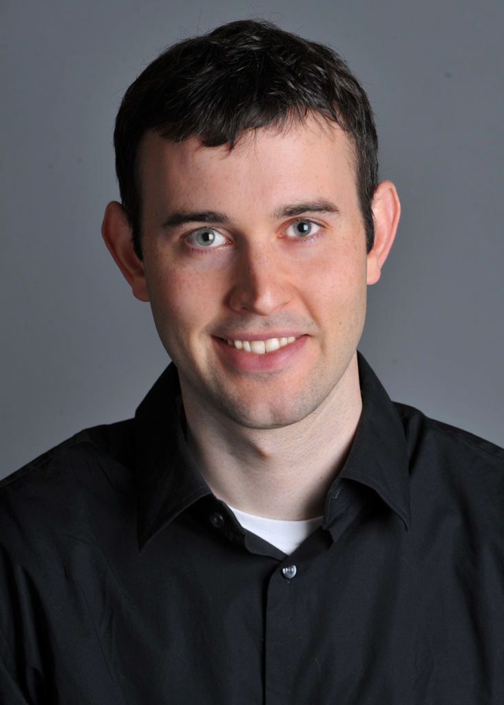
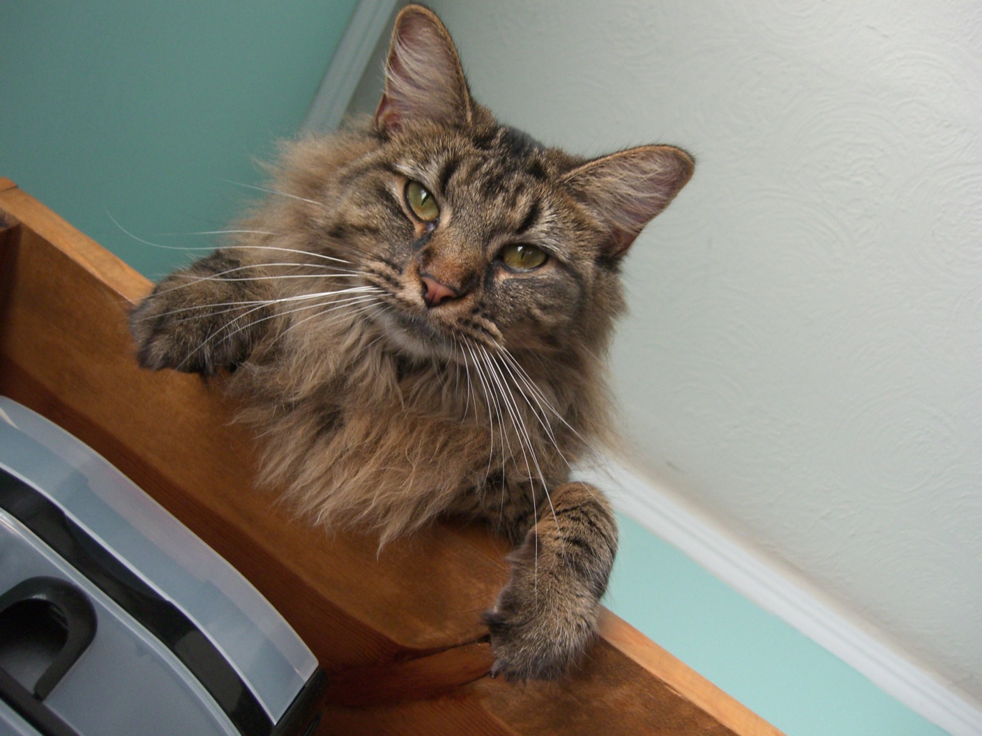
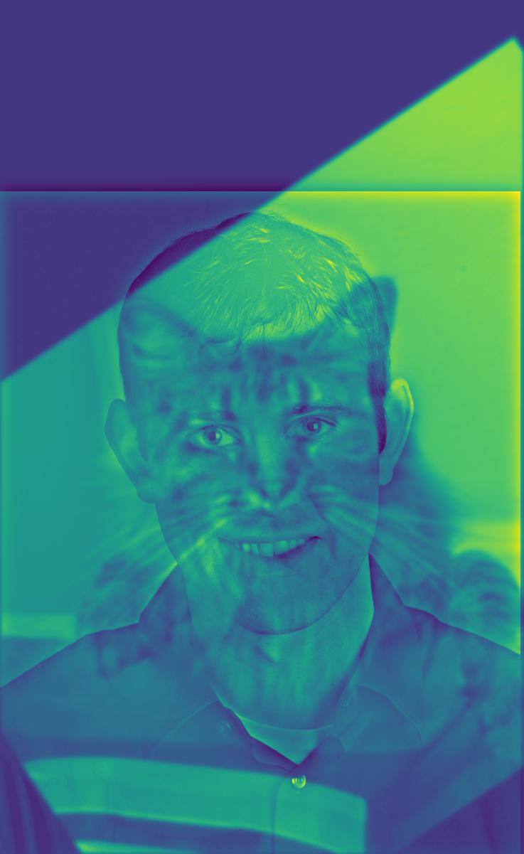
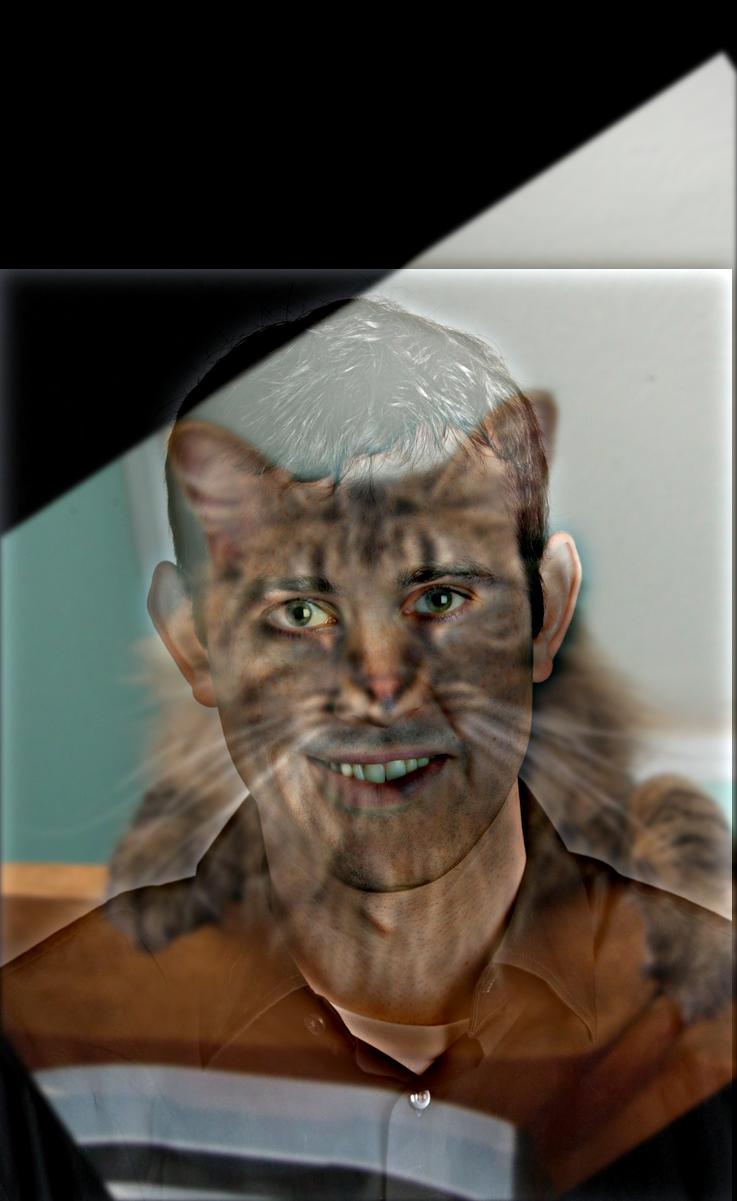
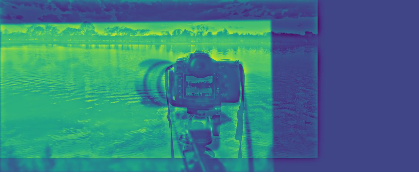
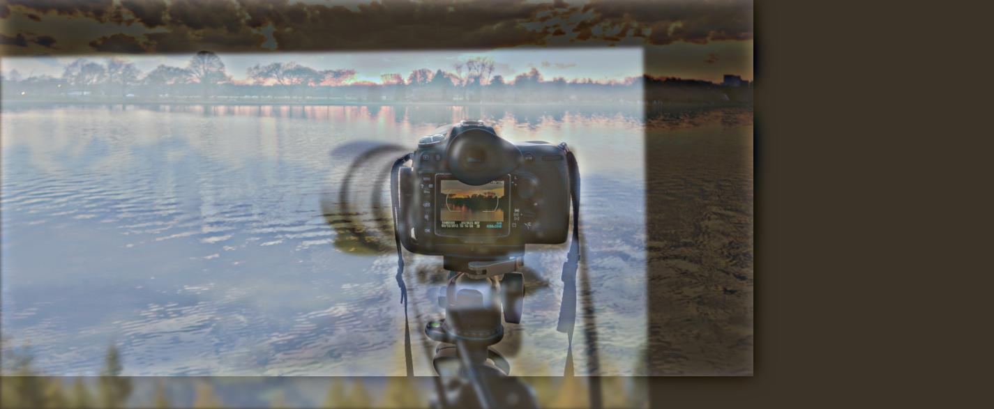
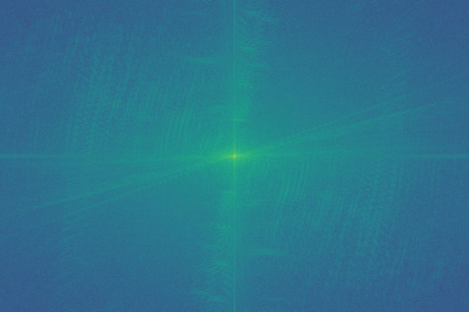
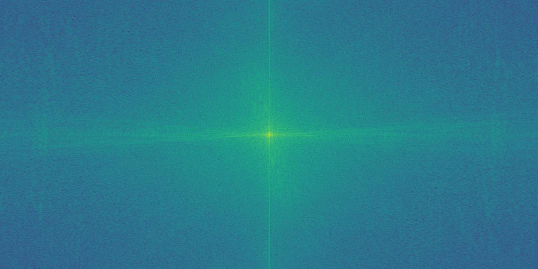
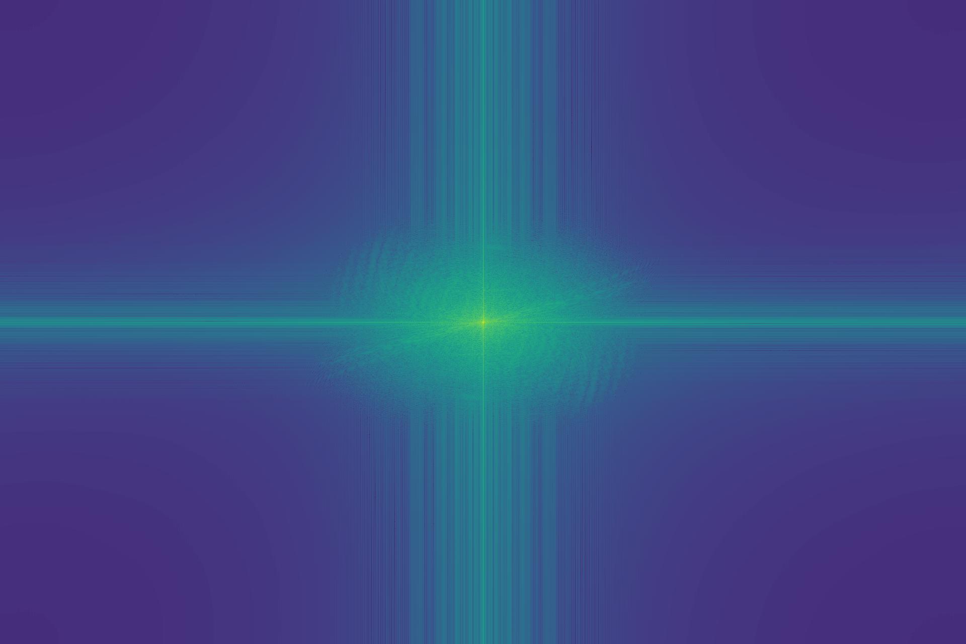
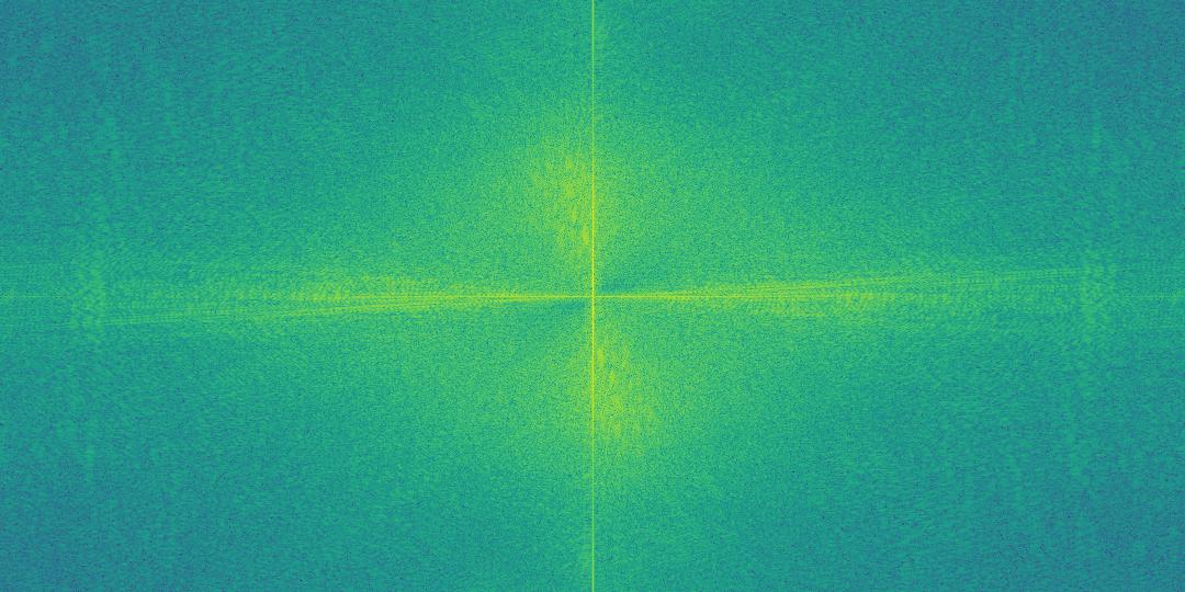
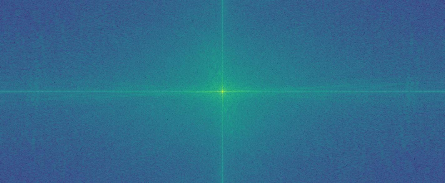
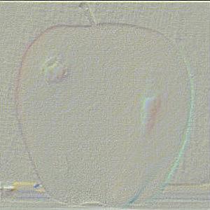
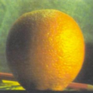
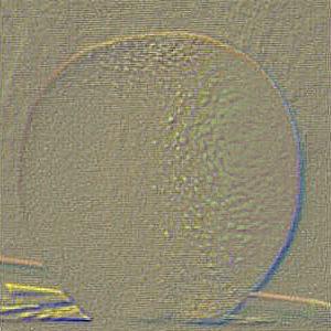
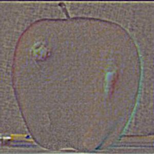
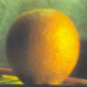
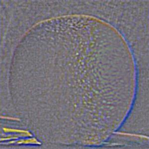
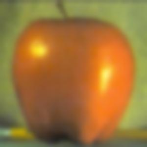
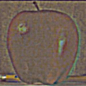
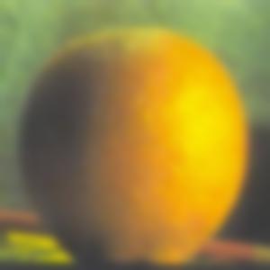
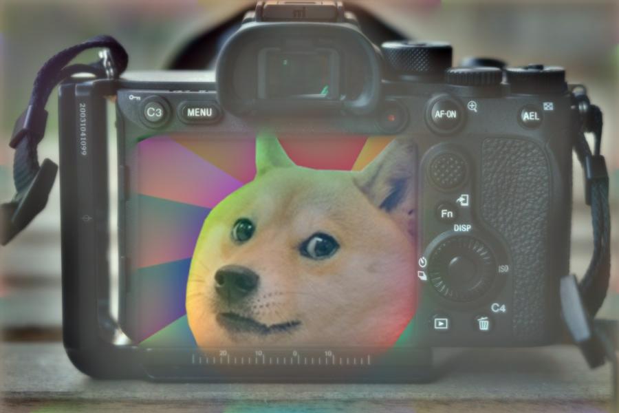
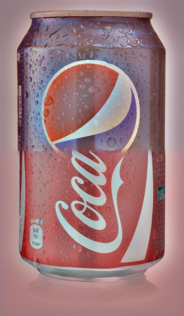
Part 2.2 Hybrid Images

Derek and his former cat Nutmeg

Derek image	cat image
hybrid greyscale image	hybrid colored image

Image of birds(?

origin im1	origin im2 / a picture I took in Monterey
hybrid greyscale image	hybrid colored image

Image of cameras

origin im1	origin im2
hybrid greyscale image	hybrid colored image

Frequency Analysis

frequency of original im1	frequency of original im2
Low pass filtered image frequency	High pass filtered image frequency
frequency of the hybrid image

Extra/Failure

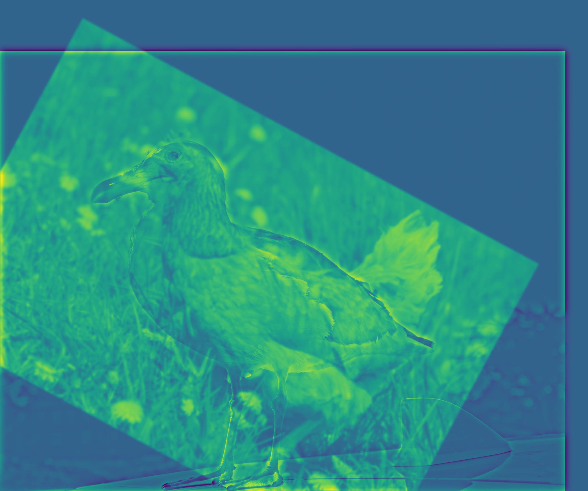
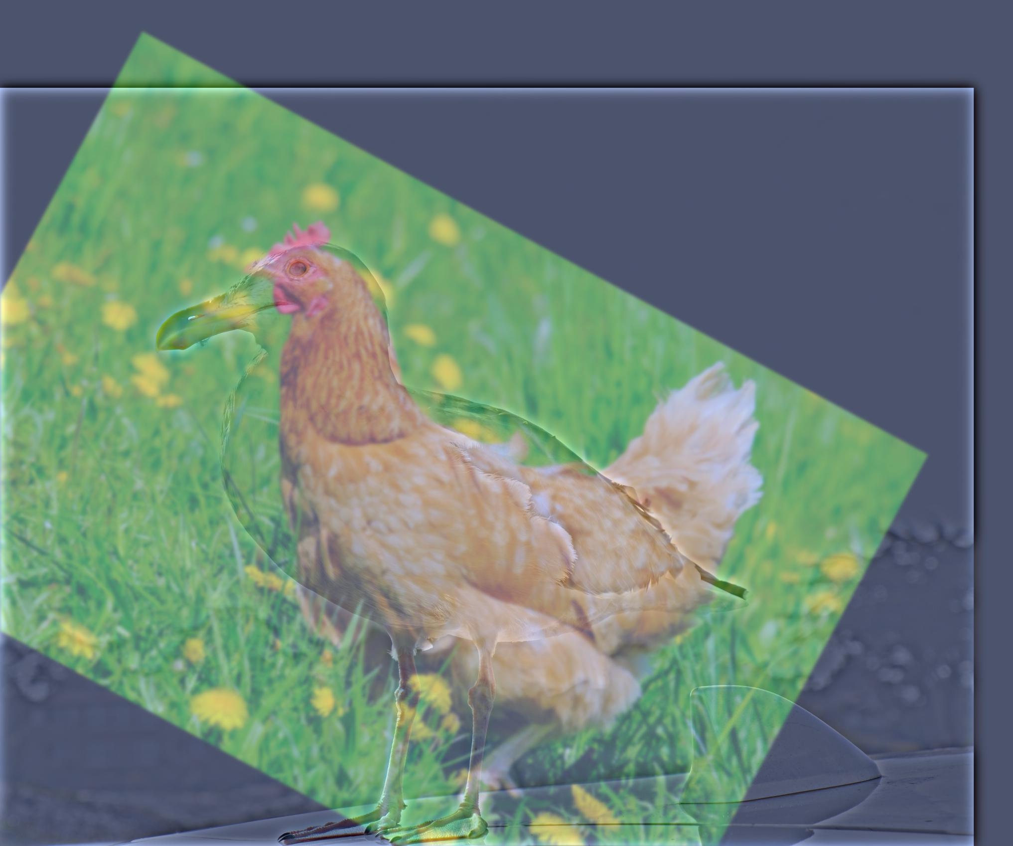
The colored image has the problem that the high pass filtered is not so visible because its color is not emphasized compared to the low pass filtered image. We would probably want the picture with a more hybrid color to be high-pass filtered, and the other picture to be low-pass filtered. We could also try to enhance the color of the high-pass filtered image.

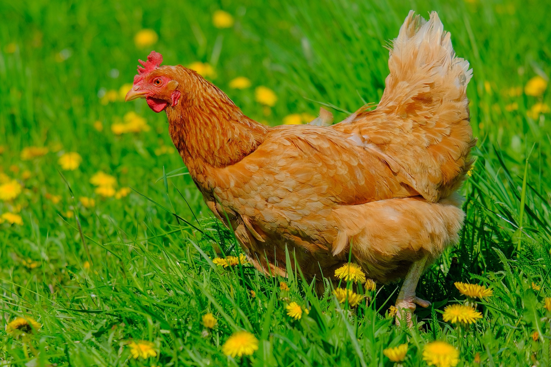
for example, in the colored bird image I showed above, because the color tone of the seagull image is kind of white, while the color tone of the chicken image is much more vivid than the seagull one, when I high-pass filter the seagull image and blend them, the seagull image is somehow hard to see. We could only see the boundary of the seagull while the color is not really obvious to viewers.

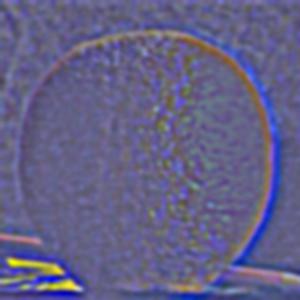
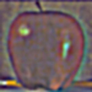
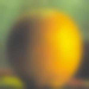
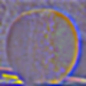
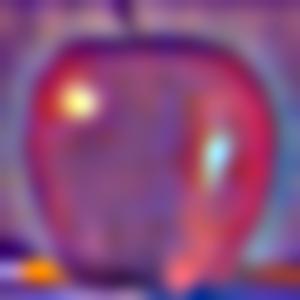
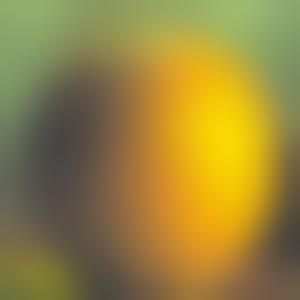
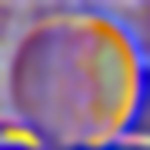
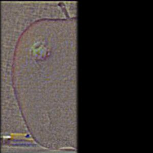
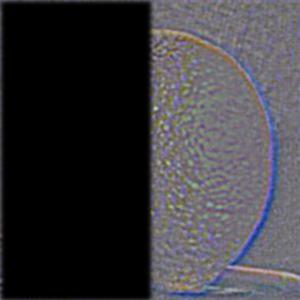
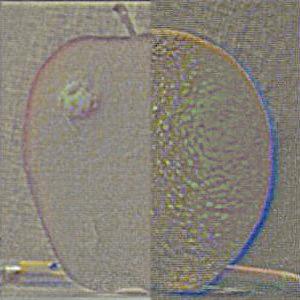
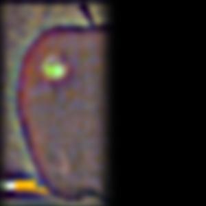
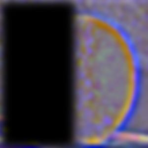
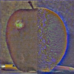
Part 2.3 Gaussian and Laplacian Stacks

apple gaussian lv0	apple laplacian lv0	orange gaussian lv0	orange laplacian lv0
apple gaussian lv1	apple laplacian lv1	orange gaussian lv1	orange laplacian lv1
apple gaussian lv2	apple laplacian lv2	orange gaussian lv2	orange laplacian lv2
apple gaussian lv3	apple laplacian lv3	orange gaussian lv3	orange laplacian lv3
apple gaussian lv4	apple laplacian lv4	orange gaussian lv4	orange laplacian lv4
apple gaussian lv5	apple laplacian lv5	orange gaussian lv5	orange laplacian lv5

Part 2.4 Multiresolution Blending

lv1 left	lv1 right	lv1 blended
lv3 left	lv3 right	lv3 blended
lv5 left	lv5 right	lv5 blended

Blended images of my choice

the original camera image	the original doge image	blended doge and camera	the binary mask used to blend the camera and the doge
the original camera image	the original doge image	blended cokepepsi	the binary mask used to blend the coke and pepsi