Fun with Filters and Frequencies
CS 194-26 Project 2 Shivam Singhal September 20, 2021
For this project, we were tasked with creating a variety of different cool images using the filtering and frequency manipulation techniques that we learned in this class.
Part 1.1: Finite Difference Operator
In this part of the project, we tried to use convolutions with different operators in order to take a see the edges in the camerman picture shown below.
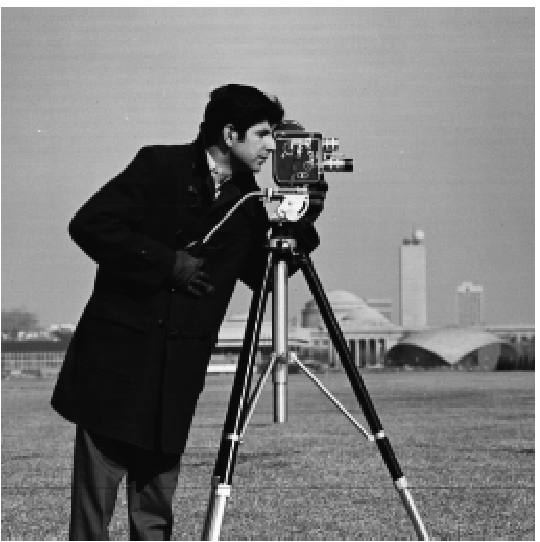
Cameraman Image
|
Below are the partial derivatives with respect to x and y that were generated by convolving the cameraman image with the following finite difference operators: [1, -1], which approximates the derivative along the x direction, and [1, -1].T, which approximates the derivative along the y direction.
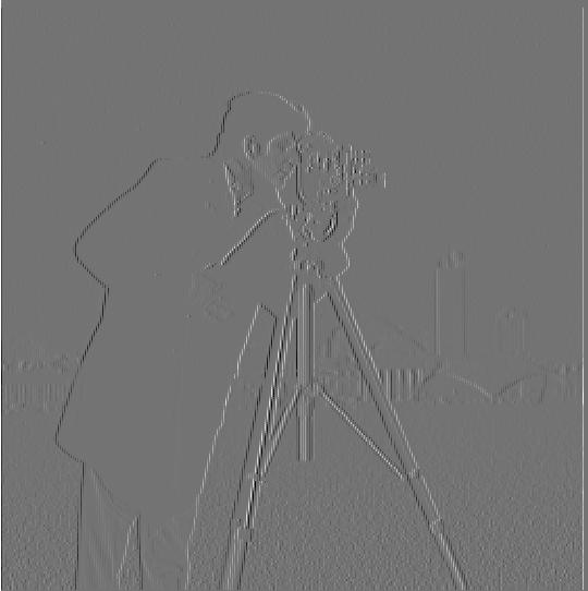
dx
|

dy
|
By performing the following elementwise computation to combine the partial derivatives, the gradient magnitude image is created: sqrt(dx^2 + dy^2). The values of the pixels in this image represent the darkness of an edge at that given location. In order to better visualize the edges, I experimented with a few thresholds to binarize the image and ended up choosing a threshold of 0.1.
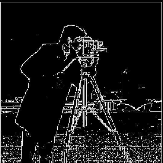
Binarized Image
|
With this technique, we can get a pretty good visual of the cameraman, but there is still quite a bit of noise.
Part 1.2: DoG Filter
To remove some of the noise from the image generated in the previous part, we can convolve the image with the Gaussian filter, which is a smoothing operator. I got the following result by creating a blurred version of the cameraman image using convolution with a gaussian and repeating the convolutions with the finite difference operators as in the previous part. The image was binarized again, and a threshold of 0.1 was used in order to get stronger edges.

Image after Applying Gaussian Blurring Method
|
In this image, we can notice that the noise is significantly reduced. Additionally, the edges are much bolder and less jagged than the edges in our previous result. We can get the same result as this method using a single convolution by convolving the gaussian with the difference operators and then applying it.
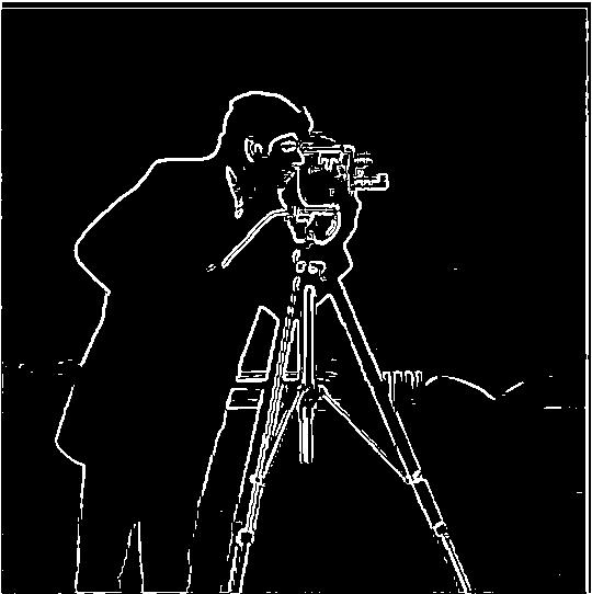
Image after Applying Single Convolution
|
Indeed, we get the same result!
Part 2.1: Image "Sharpening"
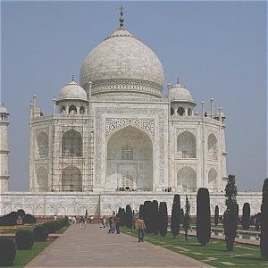
We can play around with the frequency of our images in order to make them more crisp and vivid. That is exactly what we did in this part of the project in which we were tasked with taking the following image of the Taj Mahal and sharpening it.

Taj Mahal
|
To sharpen this image, I first applied a low pass to the image using a gaussian blur and then subtracted this low pass from the original image to get the high pass.
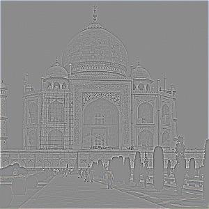
High Pass Filter
|
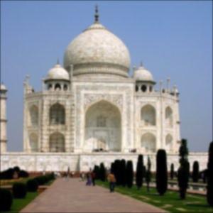
Low Pass Filter
|
I then added the high pass filter to the original image in order to sharpen it. This high pass filter is multiplied by an alpha value, which determines how much sharpening we want. For the purposes of this image, I simply chose an alpha value of 1.
Sharpened Taj Mahal
|
The sharpened image has much crisper lines around the edges of the buiding, and the trees and other greenery are definitely much more vivid. It seems like our sharpening worked! I condensed all of the filters we applied down to one filter, and I recieved the same result.
Sharpened Taj Mahal with One Mask
|
Below is my attempt at sharpening an image of our beautiful campanile. I took a normal image, blurred it using a gaussian blur, and then tried to re-sharpen it.

Blurred Campanile
|
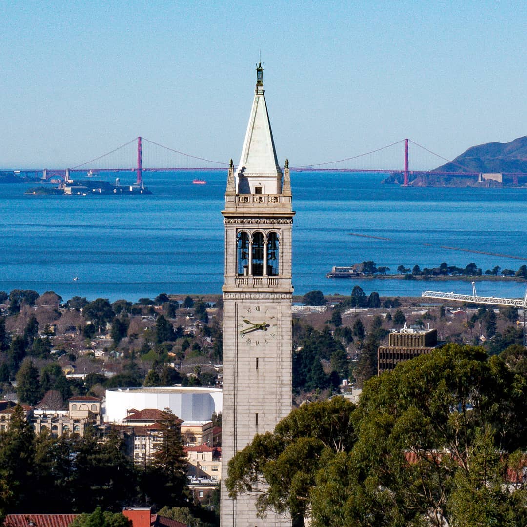
Original Campanile Image
|

Re-sharpened Campanile Image
|
As we can see, the re-sharpened campanile image doesn't quite have the definition of the original image as once we blur the image removing the high frequencies, it is difficult to get them back.
Part 2.2: Hybrid Images
Using the idea of high and low frequencies, we can create images with really interesting effects. In this part of the project, we constructed hybrid images, which are images that contain the overlay of one image's low pass and another image's high pass. If you look at the image from a distance, you will only see the low passed image, but if you look at the image close up, the high passed image will become clearer.
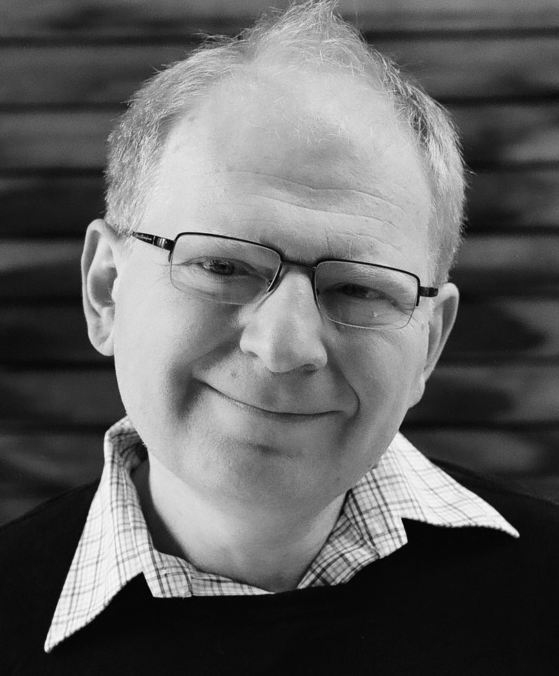
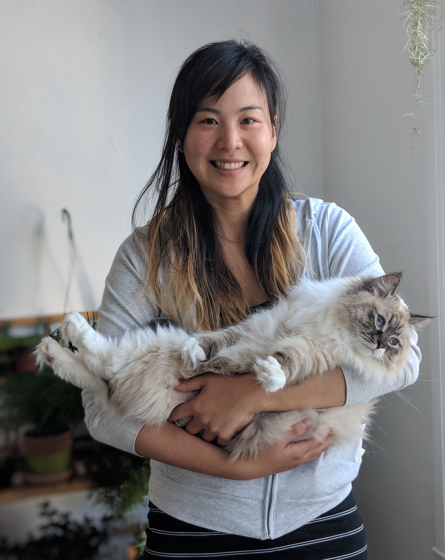
Below is the hybrid image of Derek and his cat.
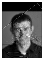
Derek and His Cat (Black-and-White)
|
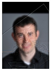
Derek and His Cat (Bells and Whistles: Color)
|
Derek is perhaps too obvious in the colored version of the image, so I would choose the black-and-white version for this image.
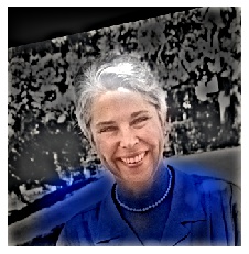
Below is the hybrid image of our two wonderful profs!. Don't they look amazing?
Prof Efros
|
Prof Kanazawa
|
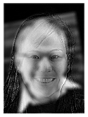
Hybrid Profs!
|
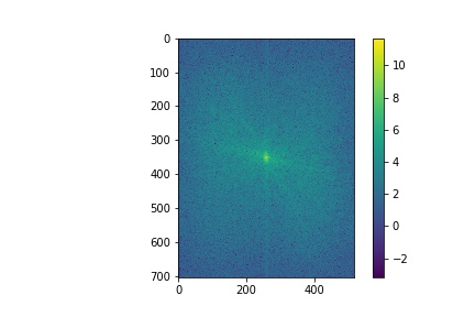
Below is the FFT analysis of the hybrid prof example.
After applying the high pass, the low frequencies from Prof Kanazawa's image are removed.
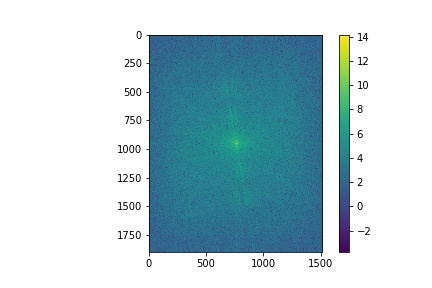
Original FFT for Prof Kanazawa's Image
|
High Pass FFT for Prof Kanazawa's Image
|
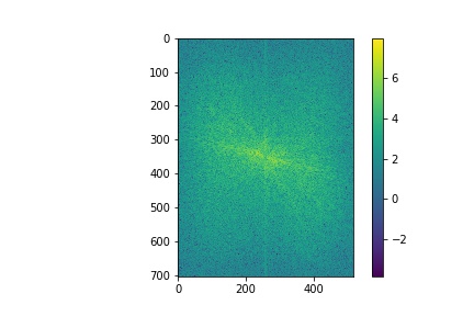
After applying the low pass, the high frequencies from Prof Efros' image are removed.
Original FFT for Prof Efros' Image
|
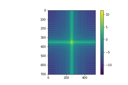
Low Pass FFT for Prof Efros' Image
|
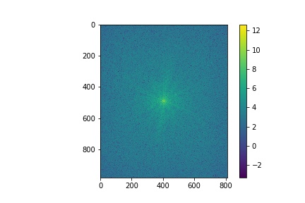
Below is the FFT of the hybrid image. We can see a combination of the Low Pass FFT and High Pass FFT in this visualization.
Hybrid Profs FFT
|
>
Below is the my attempt at creating a hybrid image of our Chancelor Christ from when she was younger and today!.
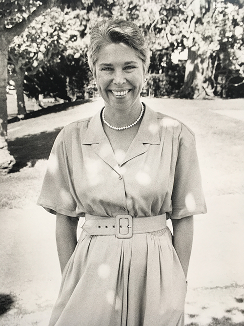
Younger Carol Christ
|
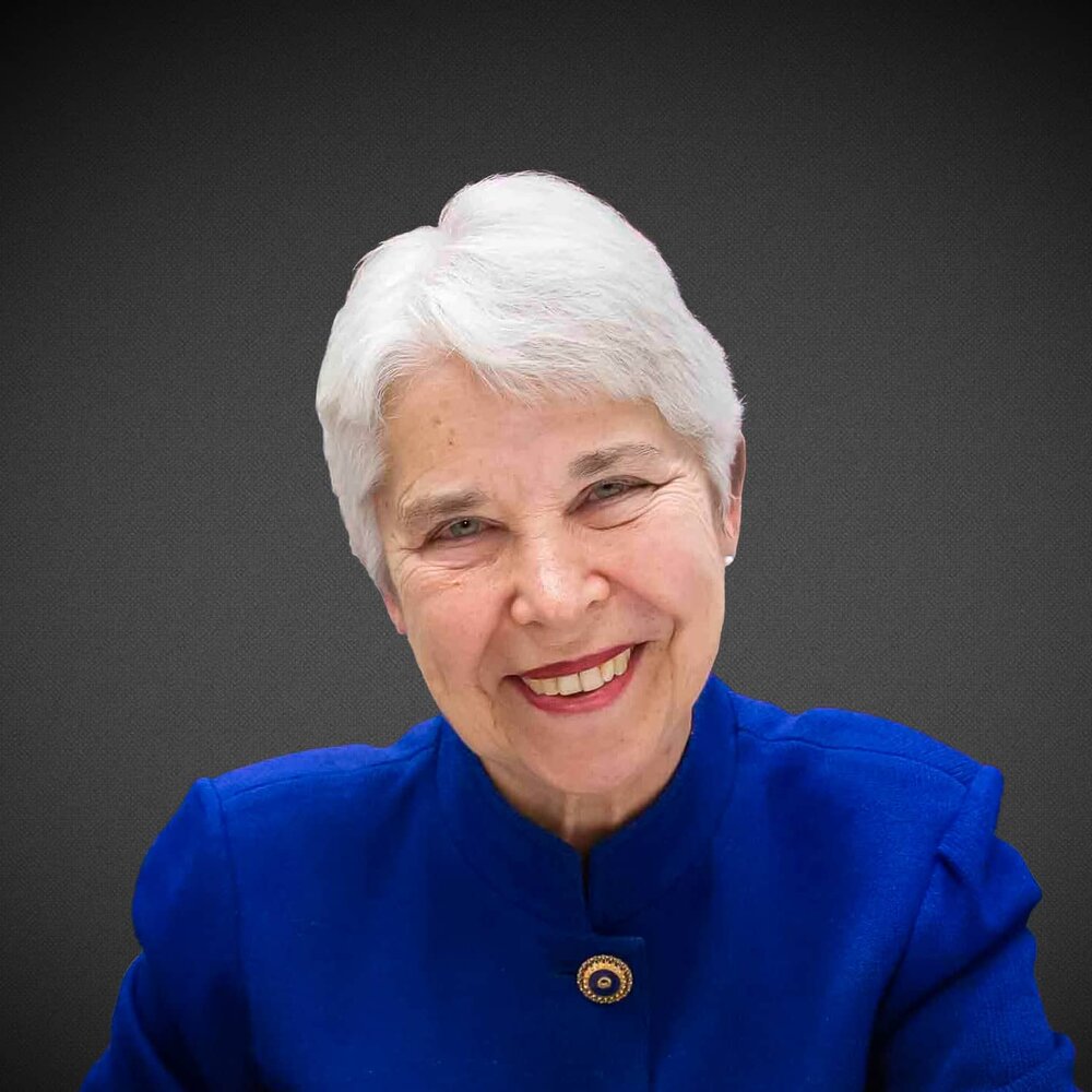
Present-day Carol Christ
|
Hybrid Carol!
|
I am not too sure if I would consider this to be a successful example, just because it seems like present-day Chancelor Christ is perhaps too hidden in the background.
Part 2.3: Gaussian and Laplacian Stacks
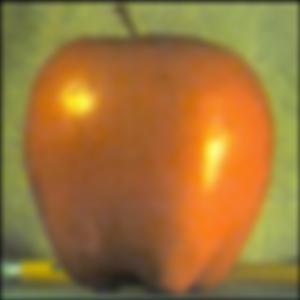
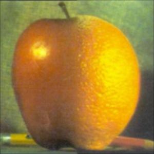
In this part of the project, we were tasked with implementing Gaussian and Laplacian stacks for the apple and orange images provided to us, so we could perform multiresolution blending.
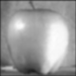
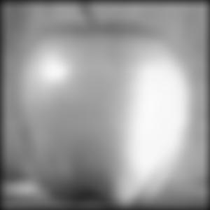
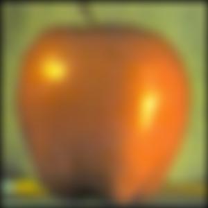
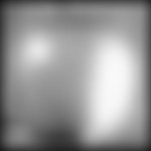
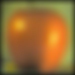
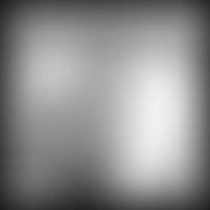
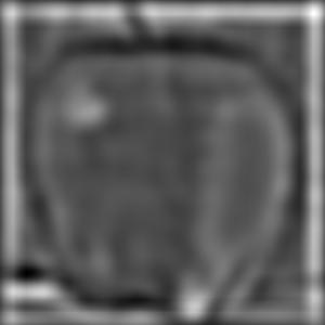
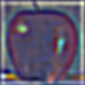
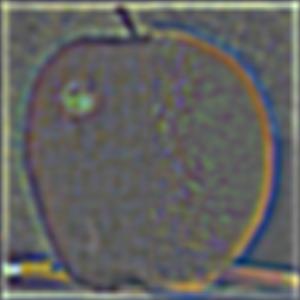
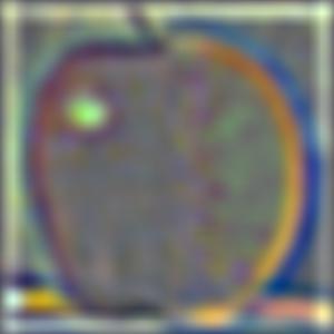
A Gaussian stack is a series of images that are blurred more as we get deeper into the set. For the purposes of this project, I chose to double the blur effect on my images for every progressive step in the stack. Below is an example of a Gaussian stack on the provided apple image in both color and black-and-white.
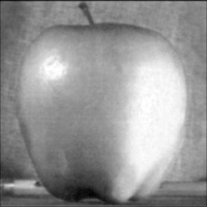
Gaussian Stack Level 1 (black-and-white)
|

Gaussian Stack Level 1 (color)
|
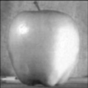
Gaussian Stack Level 2 (black-and-white)
|

Gaussian Stack Level 2 (color)
|
Gaussian Stack Level 3 (black-and-white)
|
Gaussian Stack Level 3 (color)
|
Gaussian Stack Level 4 (black-and-white)
|
Gaussian Stack Level 4 (color)
|
Gaussian Stack Level 5 (black-and-white)
|
Gaussian Stack Level 5 (color)
|
Gaussian Stack Level 6 (black-and-white)
|

Gaussian Stack Level 6 (color)
|
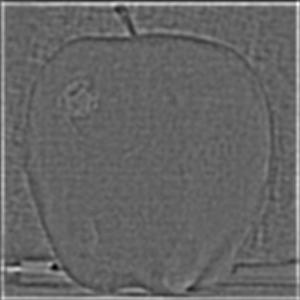
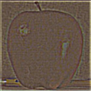
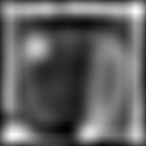
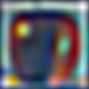
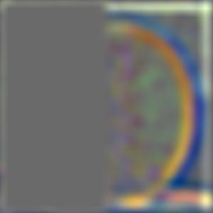
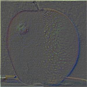
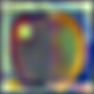
Images in the Laplacian stack represent the difference between the image at a given index in the Gaussian stack and the image at the index before it. Since the images in the Laplacian stack are supposed to add up to the original image, the last image in the stack is simply the same as the last image in the Gaussian stack. Below is an example of the Laplacian stack applied to the apple image, again in both color and black-and-white.
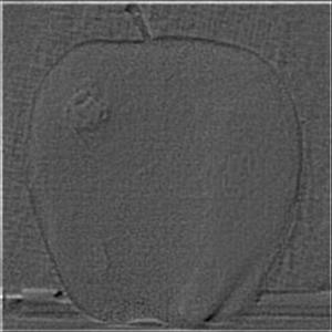
Laplacian Stack Level 1 (black-and-white)
|
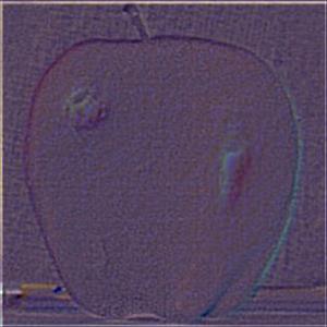
Laplacian Stack Level 1 (color)
|
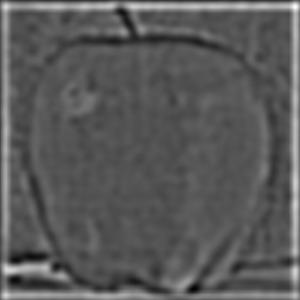
Laplacian Stack Level 2 (black-and-white)
|
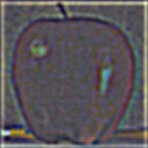
Laplacian Stack Level 2 (color)
|
Laplacian Stack Level 3 (black-and-white)
|
Laplacian Stack Level 3 (color)
|
Laplacian Stack Level 4 (black-and-white)
|
Laplacian Stack Level 4 (color)
|
Laplacian Stack Level 5 (black-and-white)
|
Laplacian Stack Level 5 (color)
|

Laplacian Stack Level 6 (black-and-white)
|
Laplacian Stack Level 6 (color)
|
More examples of the stack are shown in the next part where we construct the oraple!
Part 2.4: Multiresolution Blending (a.k.a. the oraple!)
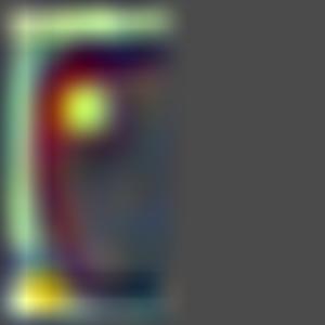
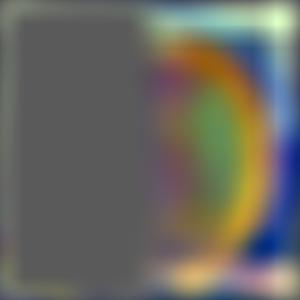
To create a fusion between the apple and orange images provided, I made use of the Gaussian and Laplacian stacks that were previously implemented. I used a progressively blurred mask in order to create a blend between the images. First, a laplacian stack was applied to both of the images, and a gaussian stack was applied to the desired mask, which in this case was simply a vertical seam. I then applied the mask to one of the images and (1-the mask) to the other image, and I proceeded to add them together. Below is a visualization of the mask being applied to the apple, the orange, and the oraple.
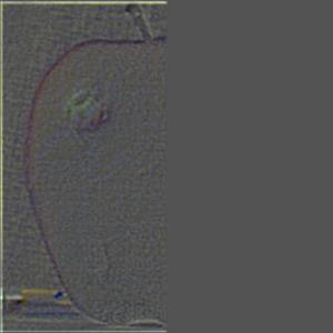
Apple Layer 1)
|
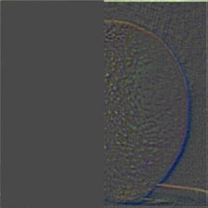
Orange Layer 1
|
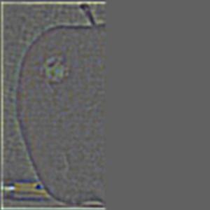
Apple Layer 2)
|
Orange Layer 2
|
Apple Layer 3)
|
Orange Layer 3
|
Apple Layer 4)
|
Orange Layer 4
|
Apple Layer 5)
|
Orange Layer 5
|
Oraple Layer 1
|
Oraple Layer 3
|
Oraple Layer 4
|
Oraple Layer 5
|
Below is the final result of all of our hard work!
The Oraple!
|
Here are some cool examples of blurring that I came up with. I first tried to combine a tunnel and a picture of heaven because there is always light at the end of the tunnel. A square filter was used for this.
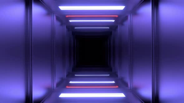
Tunnel
|
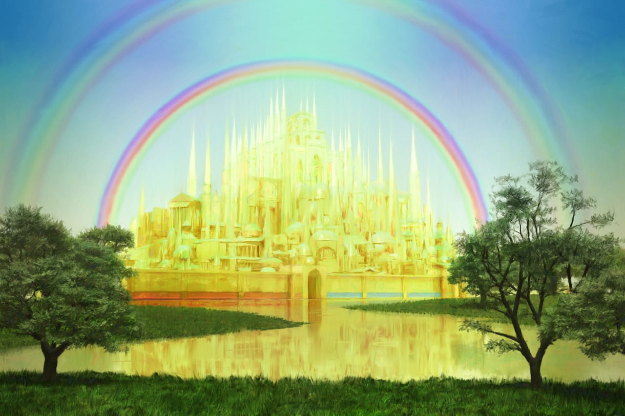
Heaven
|
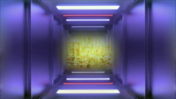
Light at the end of the Tunnel!
|
The second image I created used an oval filter to make the illusion of someone seeing an alien as they look into a telescope!
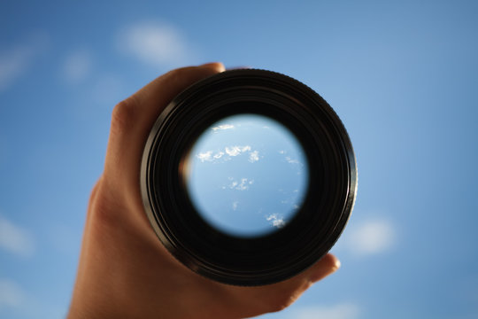
Telescope
|
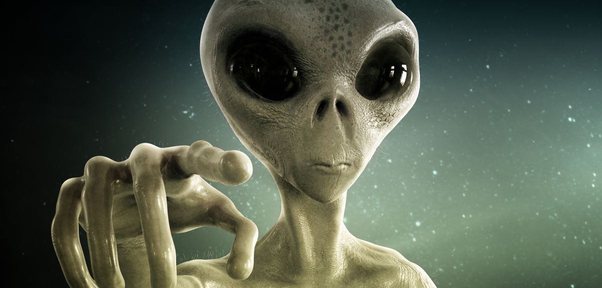
Alien
|
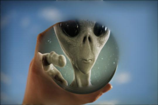
I see Aliens!
|