In this project, I used high and low frequency filtering to produce some really cool images!
Part 1.1: Finite Difference Operator
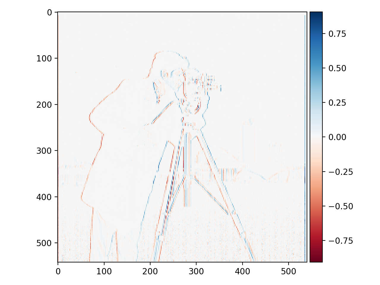
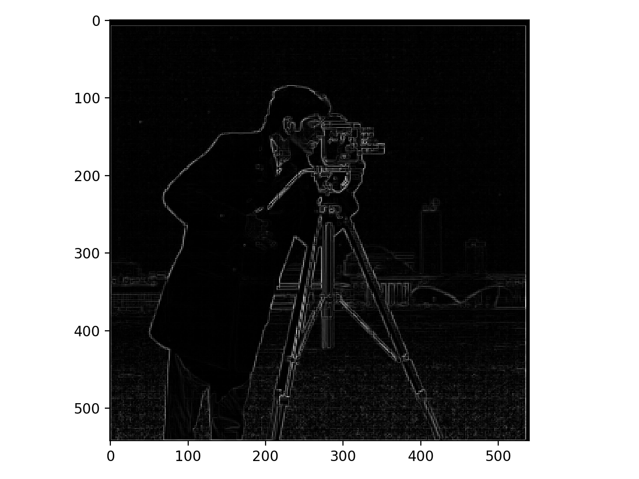
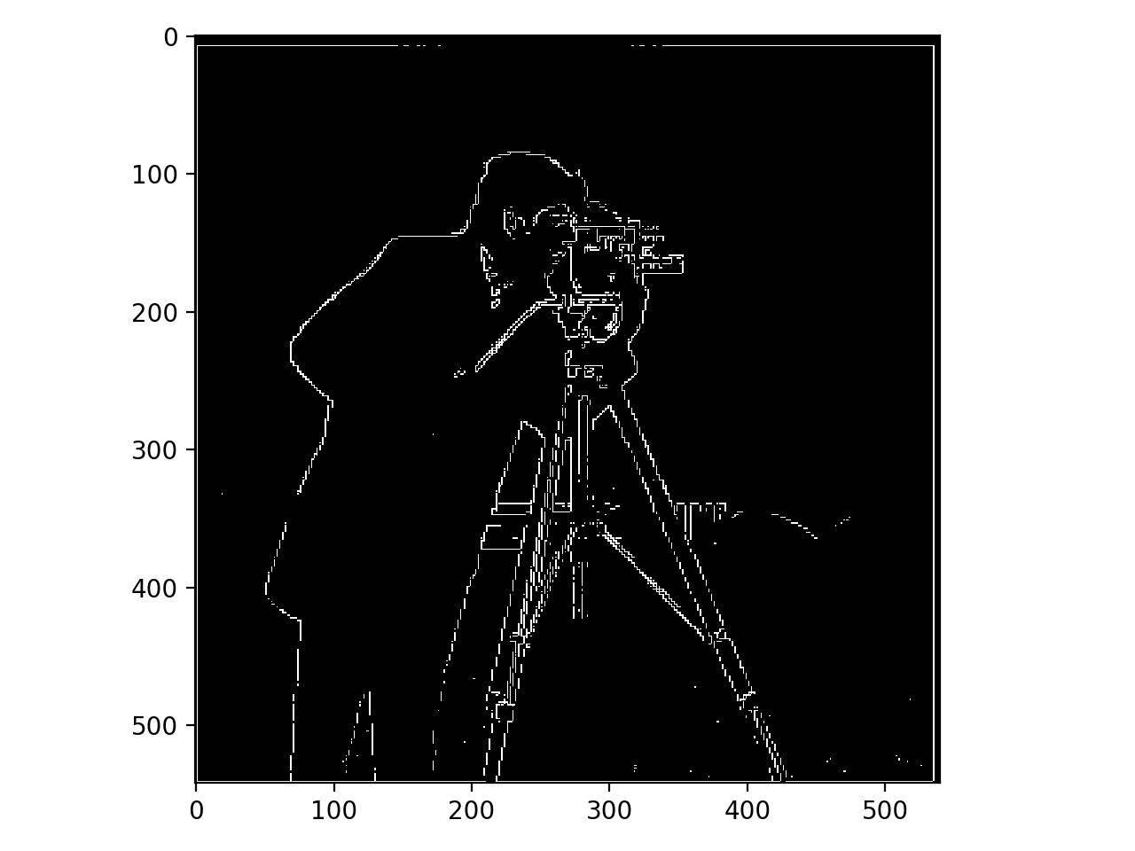
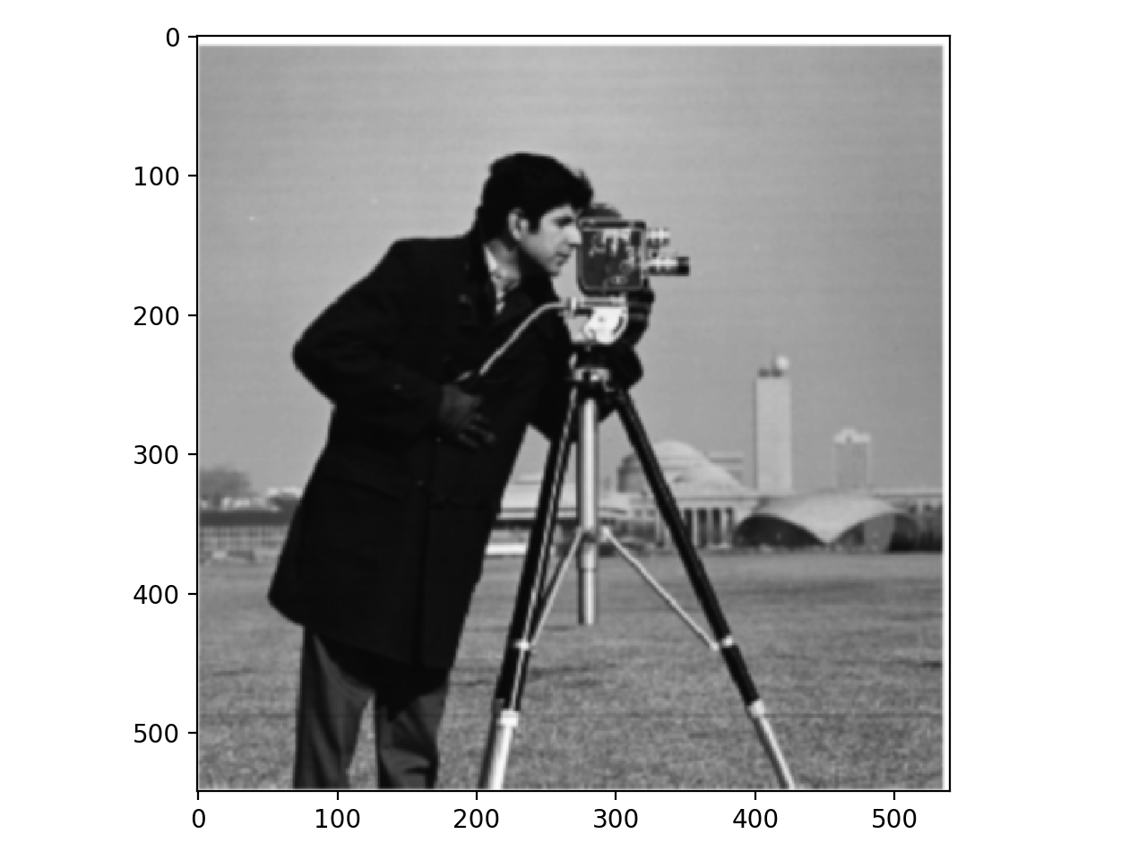
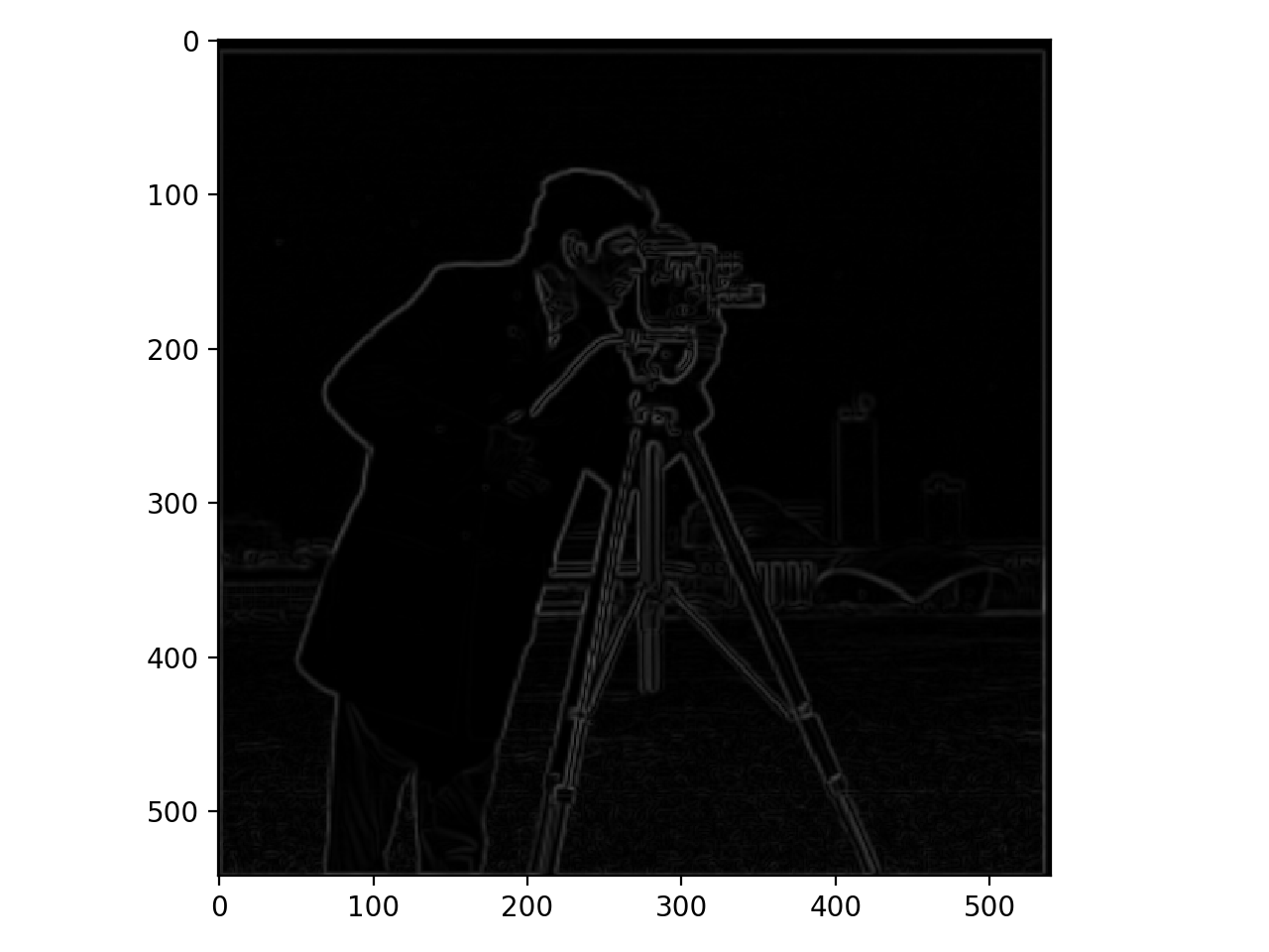
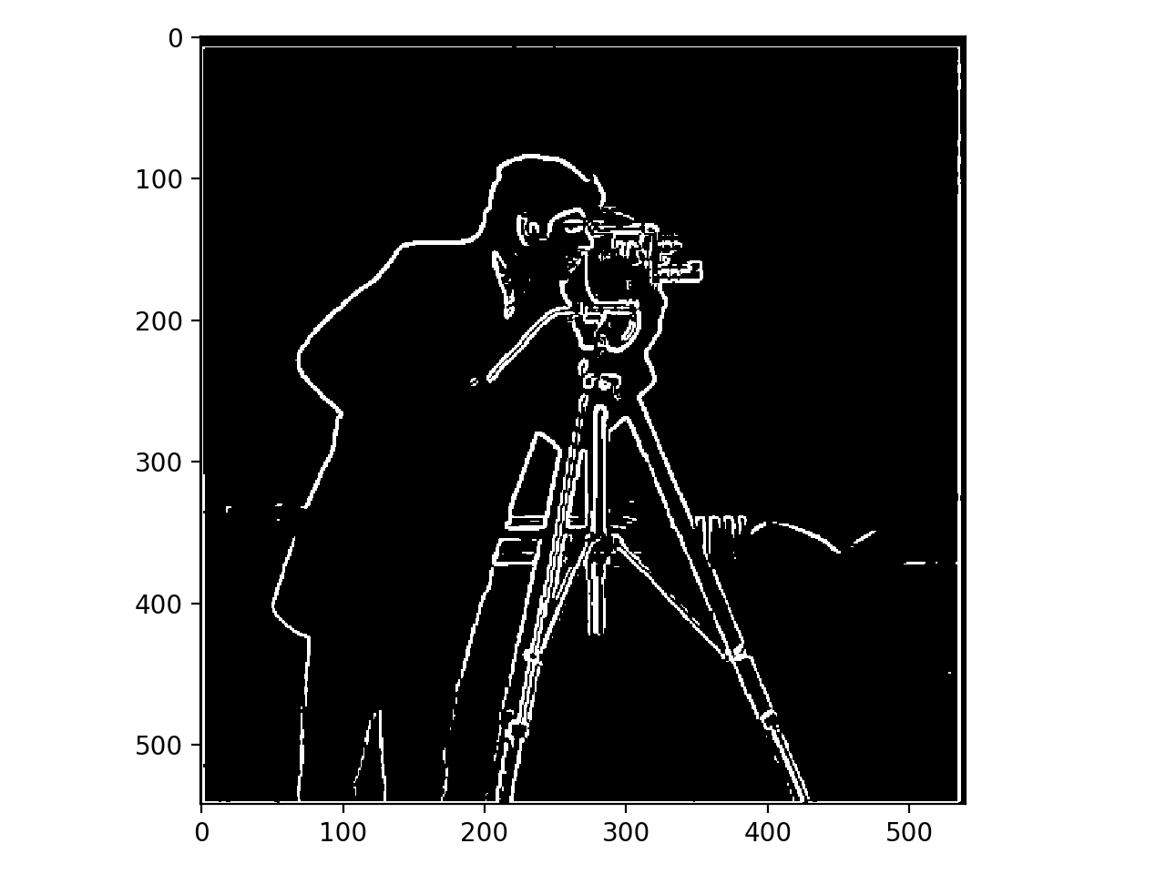
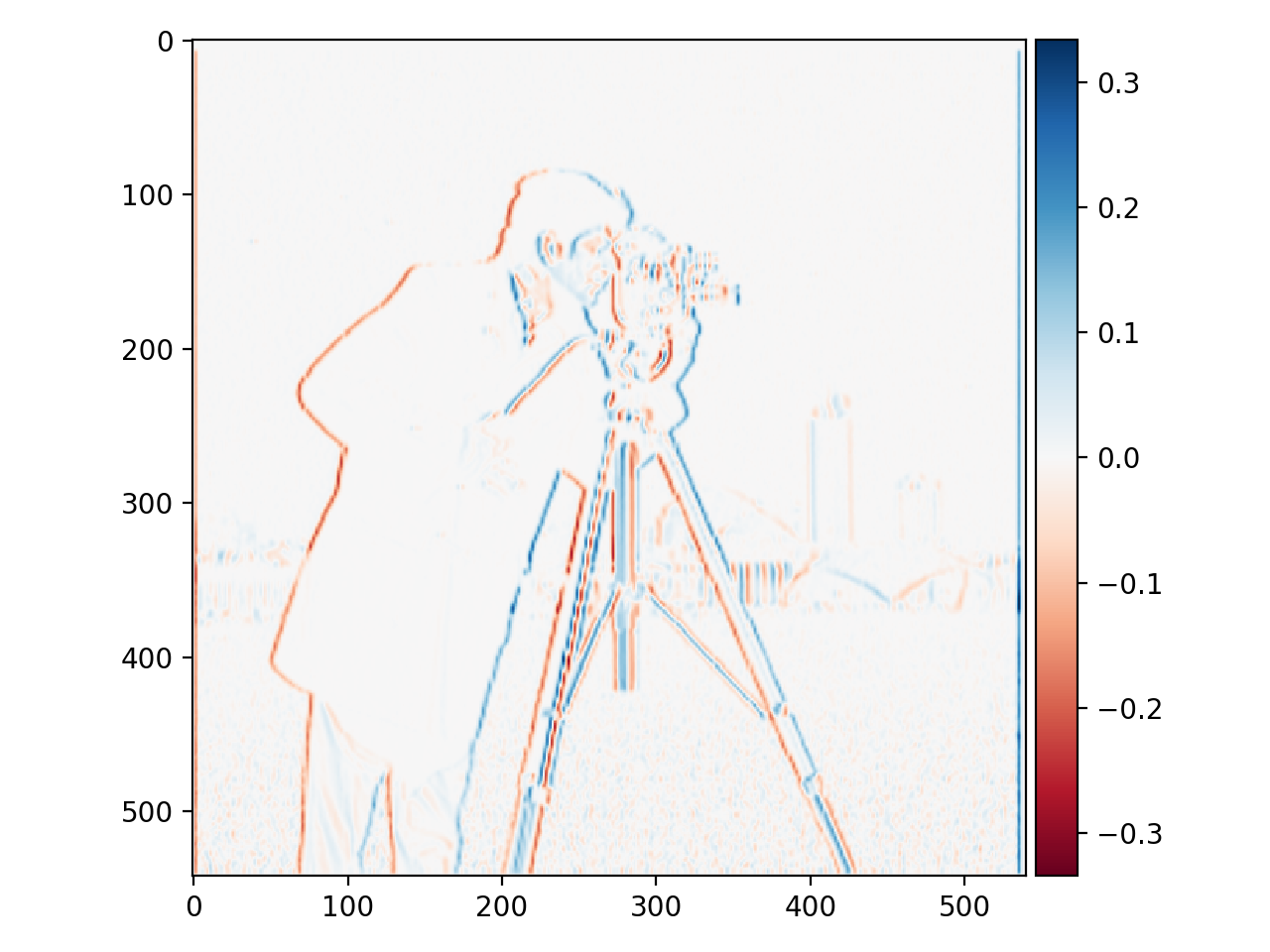
In this part, I created x and y gradient images by convolving the cameraman image with the x and y finite difference operators (Dx and Dy). These operators work by approximating the image gradient at each point as the difference between two adjacent pixel values (Dx uses adjacent x pixels and Dy uses adjacent y pixels). I then calculated the gradient magnitude image by taking the elementwise square root of the sum of the squares of the x gradient image and the y gradient image. Finally, I turned that into an edge image by applying a binary filter with a threshold of 0.3.
x gradient image y gradient image gradient magnitude image edge image (threshold = 0.3)
Part 1.2: Derivative of Gaussian (DoG) Filter
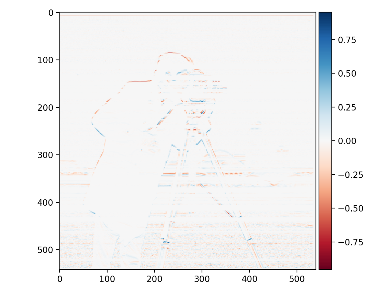
In this part, I used blurring to improve the noise in the edge image from part 2.1. To create the blurred image, I convolved the cameraman image with a gaussian of kernel size 5. Then, I applied the same steps as in part 2.1 to get the edge image. My results are shown below.
cameraman blurred cameraman blurred convolved with D_x cameraman blurred convolved with D_y gradient magnitude image edge image (threshold = 0.1)
Applying the Dx and Dy convolutions after blurring the image helped reduce a lot of the noise in the gradient images and therefore the edge image. I also noticed that the edges appeared thicker in the smoothed image, and they also appeared thicker in the edge image produced from the smoothed image. The max magnitude of the x and y gradients was larger with the non-smoothed image, but the average gradient magnitude was higher for the smoothed image.
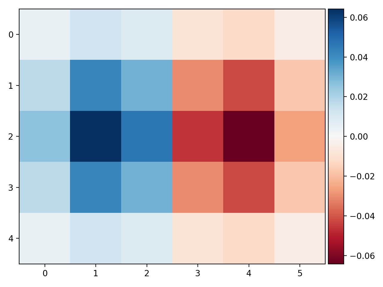
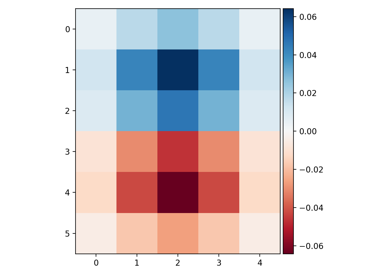
I also tried combining the Dx and Dy convolutions with the gaussian convolution, for which my results are shown below.
gaussian convolved with Dx gaussian convolved with Dy cameraman convolved with gaussian_D_x cameraman convolved with gaussian_D_y gradient magnitude image edge image (threshold = 0.1)
I ended up with the exact same results as I had when applying the convolutions separately.
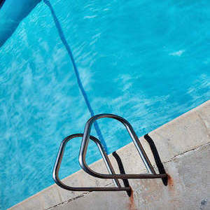
Part 2.1: Image "Sharpening"
In this part, I convolved images with the unsharp mask filter to make them appear sharper. The way this filter works is by adding some constant alpha times the image to the image, then subtracting alpha times the image convolved with a gaussian (I used a gaussian of kernel size 5, and alpha = 1). These operations can be combined into one convolution. This essentially adds more of the high frequency parts of the image to the image (the high frequency parts are obtained by subtracting the low frequency parts from the image).
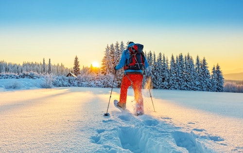
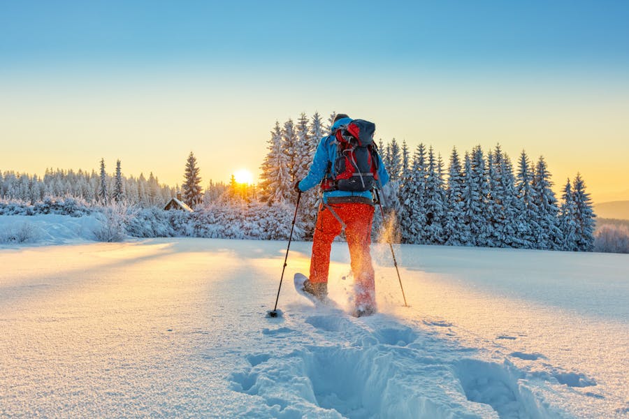
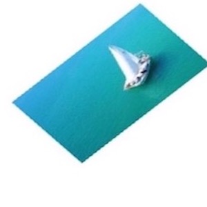
For the snowshoe image, I also tried blurring it and sharpening the blurred image to see if I would end up with the original image.
Blurred snowshoe.jpg
Sharpened blurred snowshoe.jpg
The sharpened version of the blurred image is sharper than the blurred image, but it not quite as sharp as the original image. This is probably because some information is lost in the blurring/resharpening process. When we sharpen, we are not actually getting new information and adding it to the image (all we are doing is enhancing the high frequencies), so we can't get back the original image from the blurred image by sharpening it.
Part 2.2: Hybrid Images
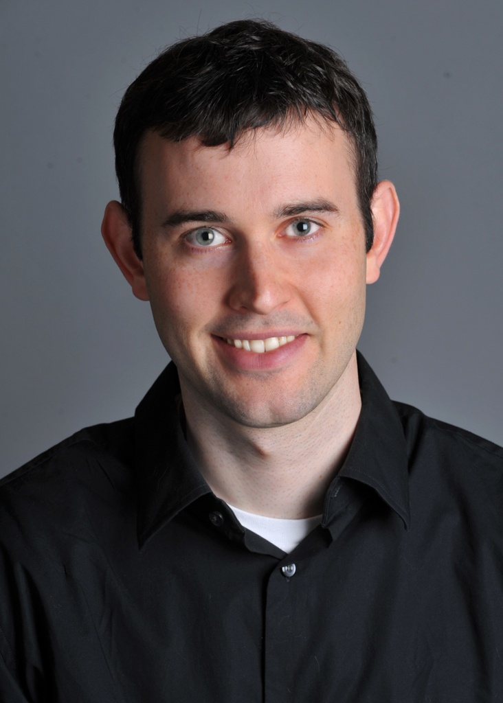
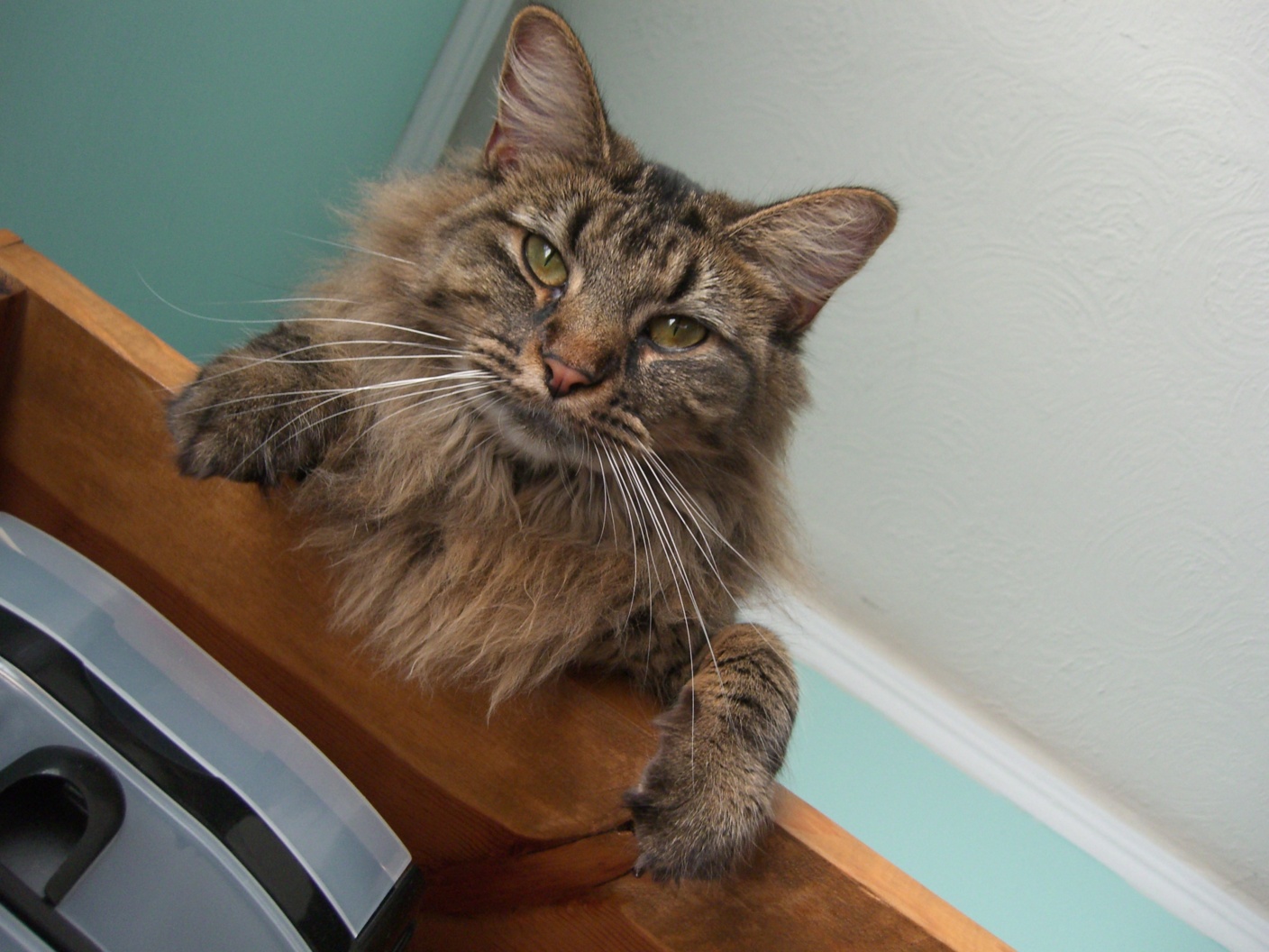
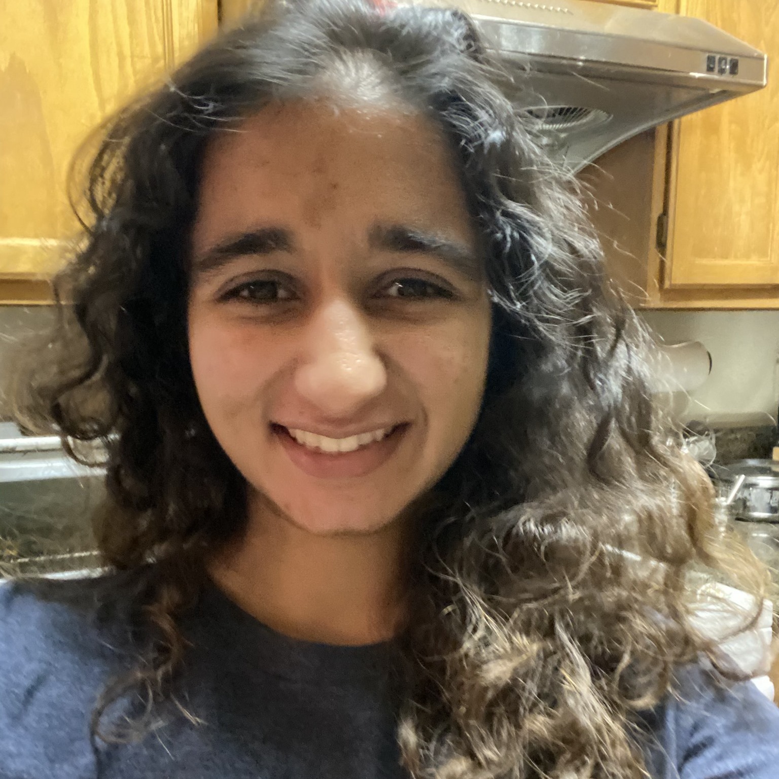
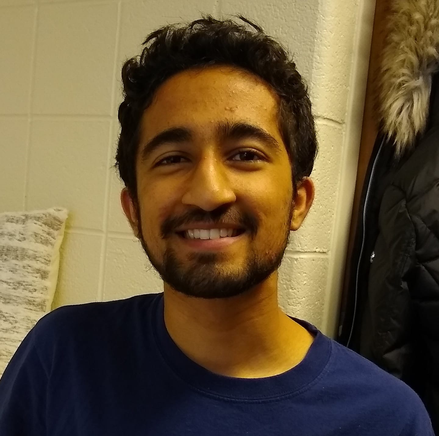
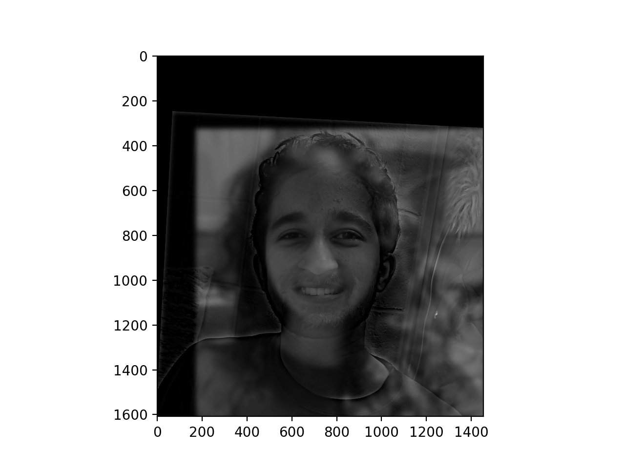
This was my favorite part of the project! For this part, given a pair of images, I extracted the high frequency part of one image and the low frequency part of the other. Then I averaged these together. When you look at the result from far away, you see the image that I took the low frequency components from. When you look at it from close up, you see the image I took the high frequency components from.
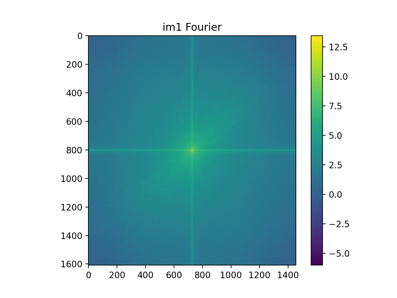
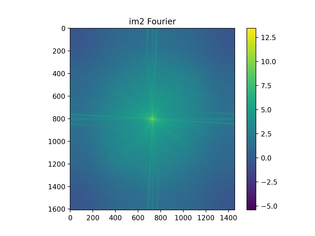
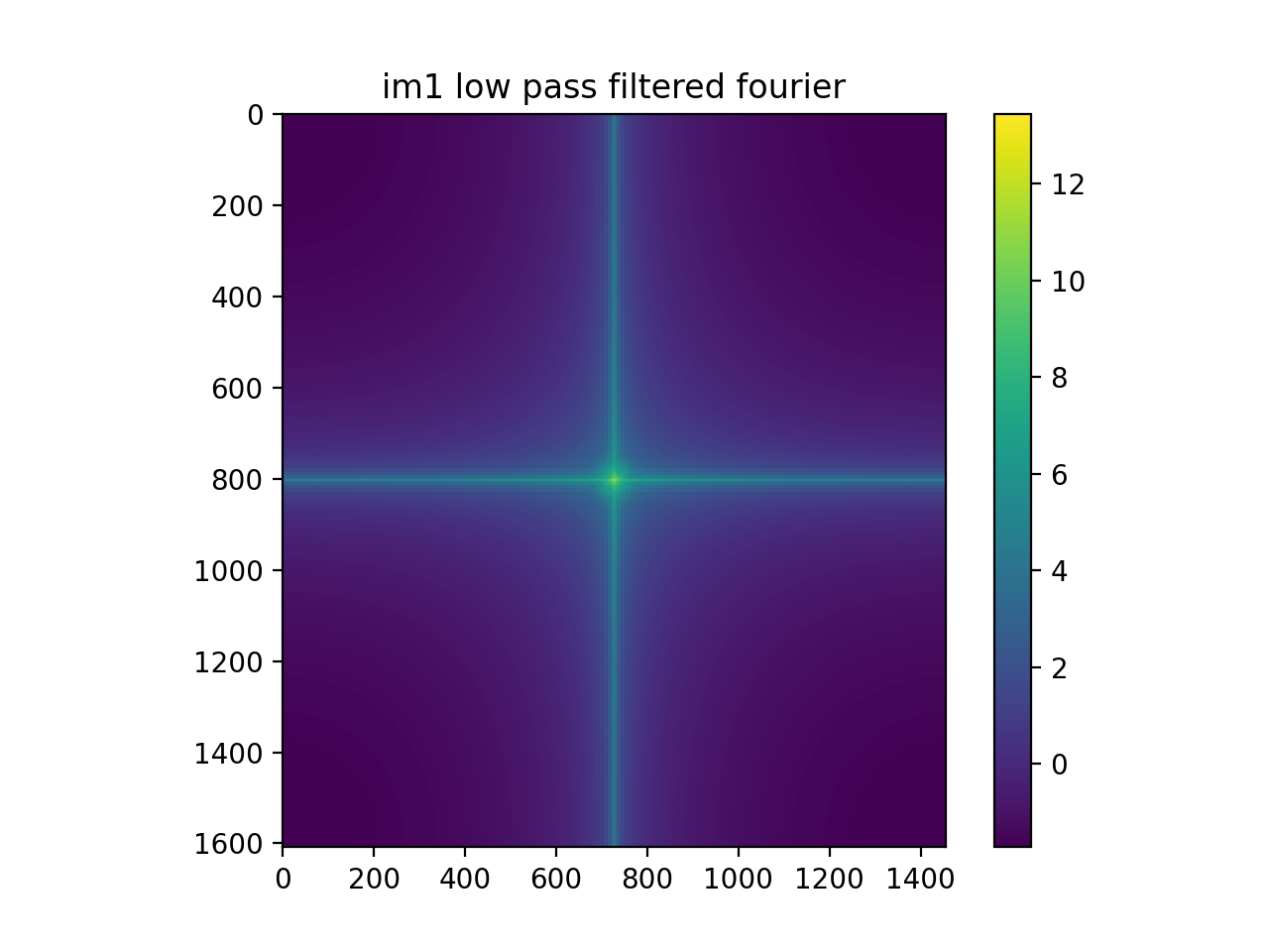
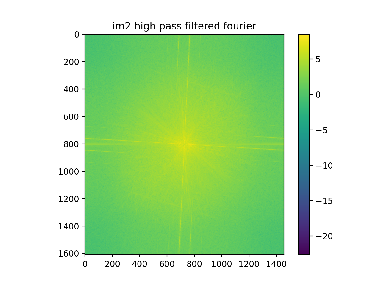
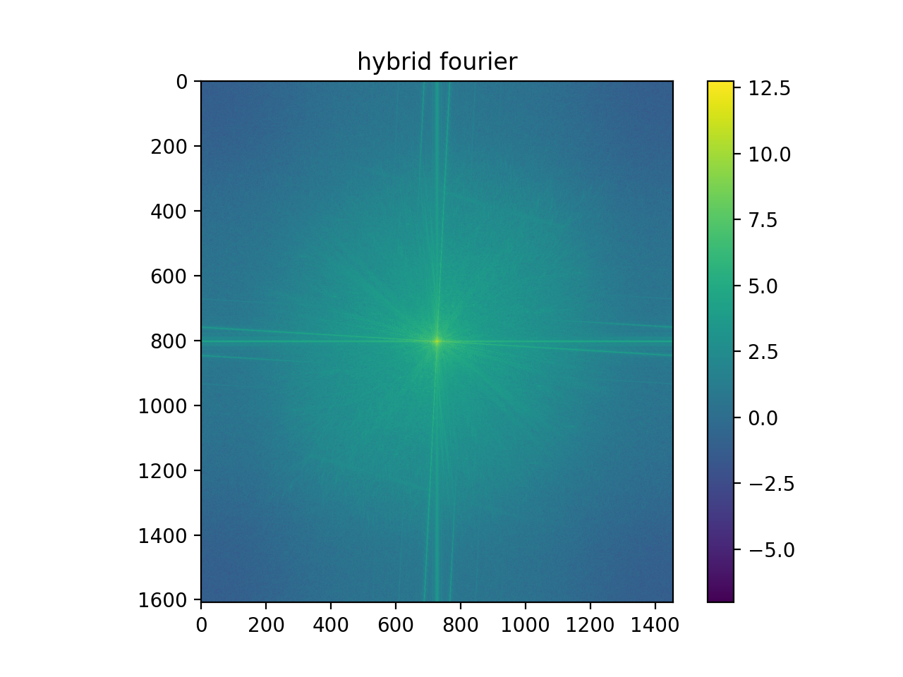
For the last set of images, I also display the fourier transforms of the input images, the filtered images, and the hybrid image.
Picture of mePicture of me fourier transform Picture of my brother Picture of my brother fourier transform My fourier transform after applying low pass filter. Most of the high frequencies have been removed, but we can see by the horizontal and vertical lines passing through the origin that the filtering was not perfect. My brother's fourier transform after applying high pass filter. The low frequencies have decreased, but were not removed completely. Hybrid picture fourier transform. It contains the high frequencies from my brother's image and the low frequencies from my image. Hybrid Siblings Picture
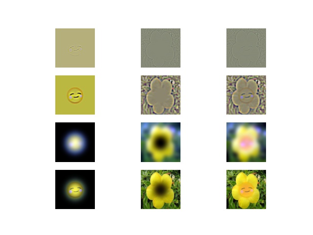
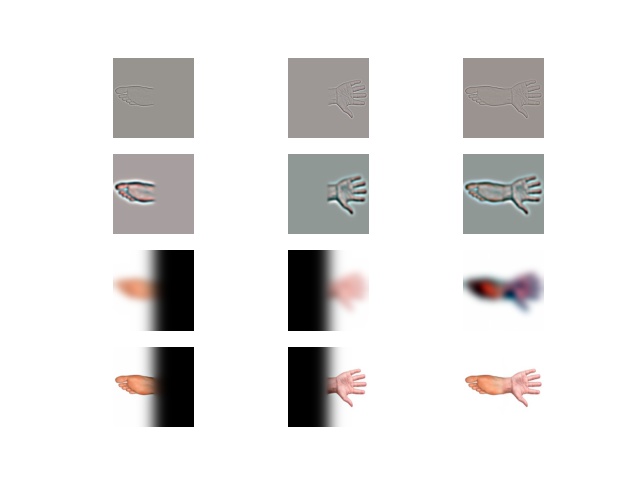
Part 2.3/2.4: Gaussian and Laplacian Stacks, Multiresolution Blending
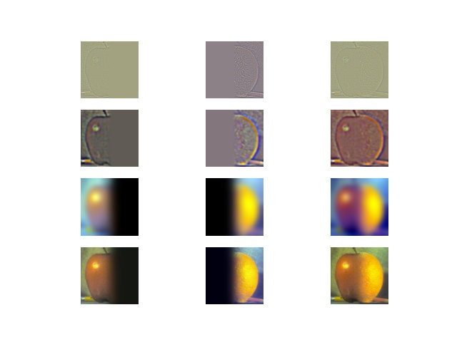
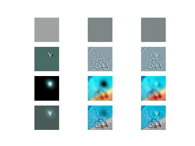
In this part of the project, our goal was to blend two images together seamlessly. To do this, I first created Gaussian and Laplacian stacks for each of the two images (the Laplacian stack contains the different frequency components of the image). The stacks were of length 5, and to create them I used a Gaussian kernel size of 11. Then, I created a mask for the part of the first image I wanted to include, and created a Gaussian stack of that mask (length 5, kernel size 21). Then, I weighted the different layers of the two Laplacian stacks by the mask gaussian layer and (1 - the mask gaussian layer) respectively. Finally, I summed the results for each layer and then summed over all the layers to get the blended image. This process works because the lower frequency Laplacian layers are weighted by a larger Gaussian, so they get blended more, and the opposite is true for the highest frequency Laplacian layers.
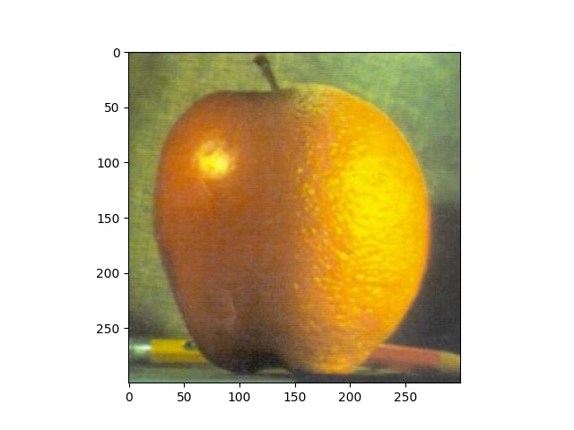
Results for the oraple:
Apple Orange Blending Process
The first 3 rows represent the 0'th, 2'nd, and 4'th layers of the Laplacian stacks, weighted by the relevant layers of the mask gaussian stack. The last row is the sum of the weighted laplacian layers. The first column is the apple, the second column is the orange, and the third column is the sum of the first two columns. The bottom right corner is the final blended result.
Blended Apple + Orange, with Mask = Half 1's on Left Side and Half 0's on Right Side
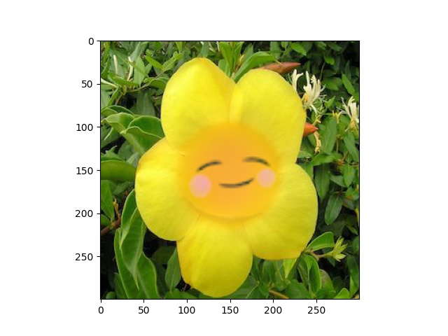
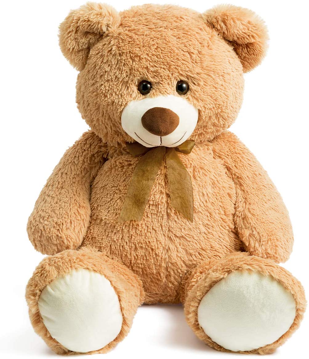
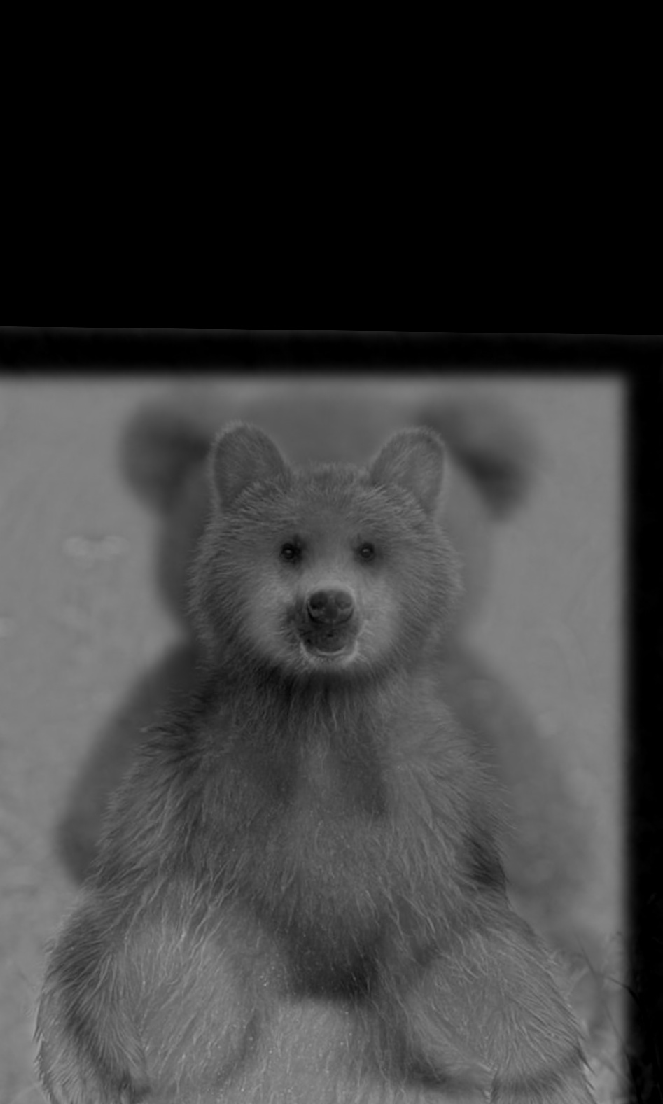
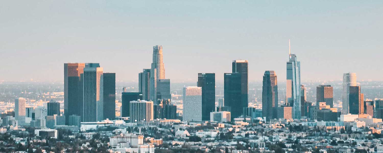
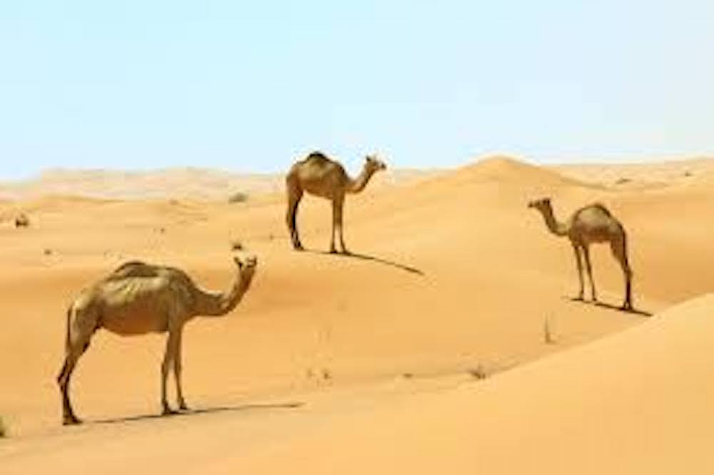
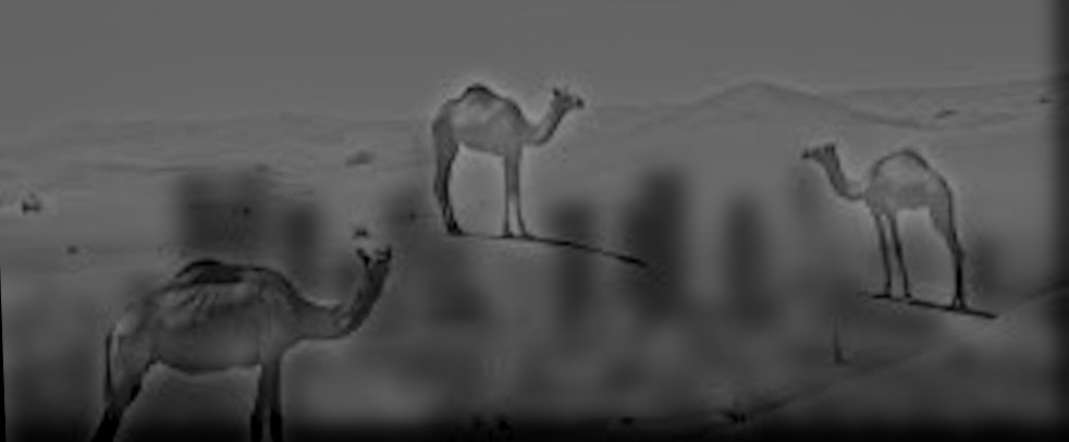
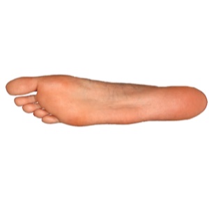
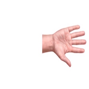
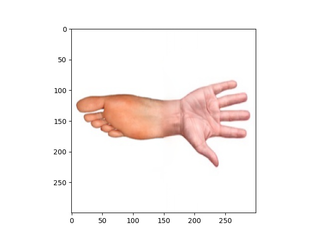
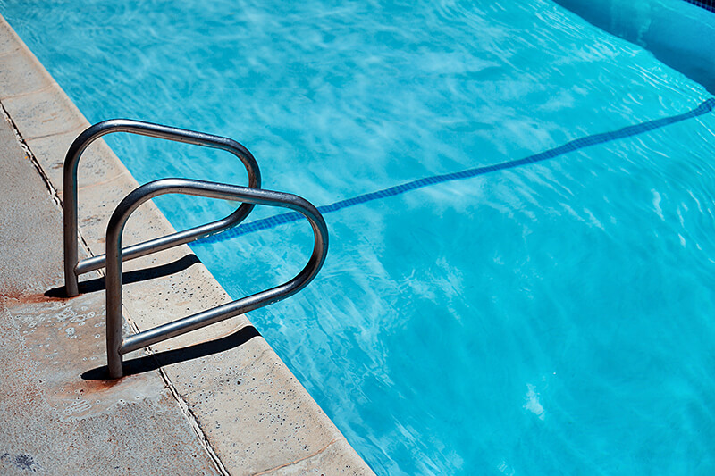
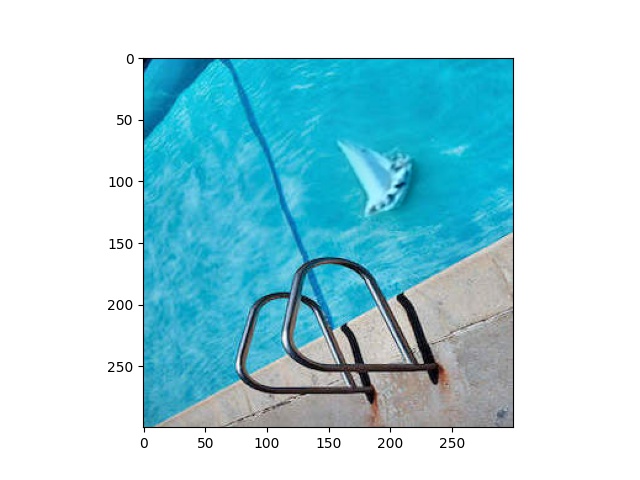
Below, I show the results for three other sets of images.
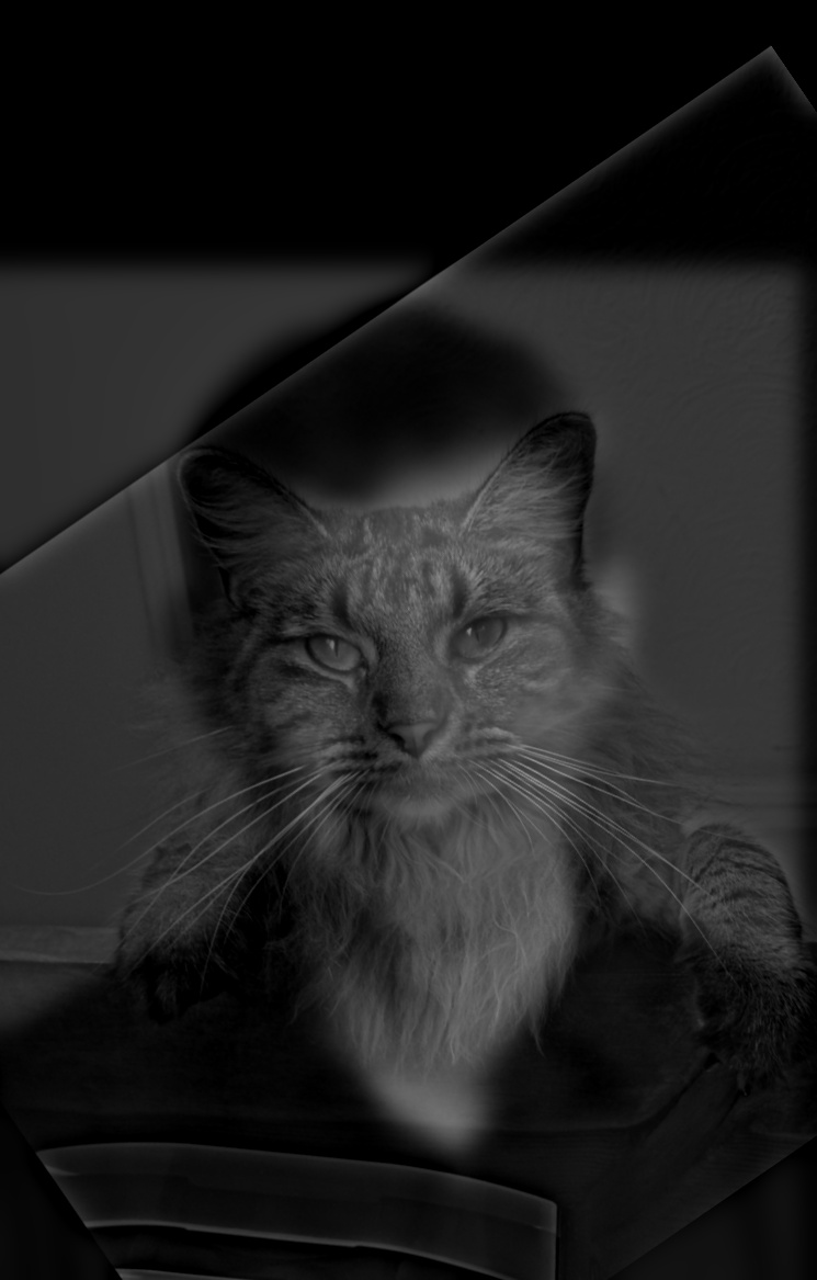
I think the result turned out okay here as well, but it would have worked better if I was blending two things with more similar shapes.
Reflection
The most important thing I learned from this project is that images are actually made up of many layers of different frequencies, and that each frequency layer differently affects how we perceive an image. For example, low frequencies are what we see from far away, and we perceive high frequencies as image sharpness. Overall, I think this was a really fun project to work on.


