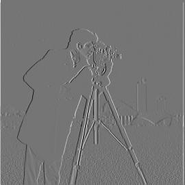
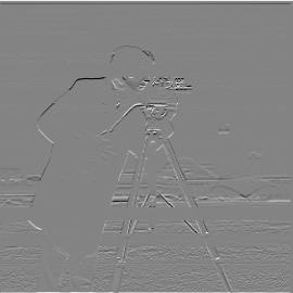
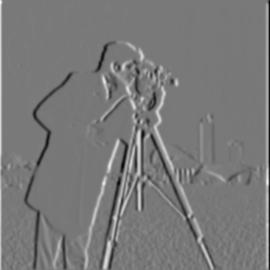
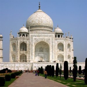
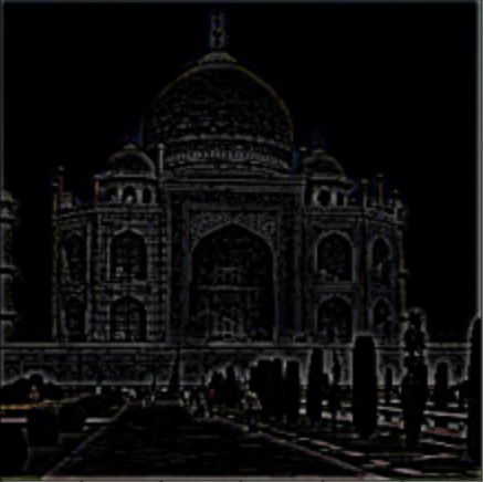
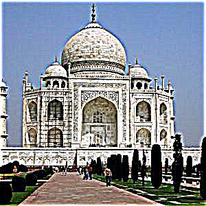
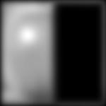
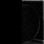
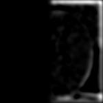
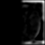
The finite difference filter was used for both the x (Dx = [1 -1]) and y (Dy = [1 -1]T) dimensions. These filters can then be convolved with an image (scipy.signal.convolve2d) to find the partial derivative with respect to both x and y for the image. This will give us the gradient of the image for both the x and y dimension. Another way to think of partial derivatives for images is to equate dx with vertical edges (as a large change in adjacent pixels along the x axis would suggest a vertical line) and dy with vertical edges (as a large change in adjacent pixels along the y axis would suggest a horizontal line). A sample image and it's vertical and horizontal edges, which were found through the finite difference filters, are shown below.
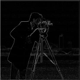
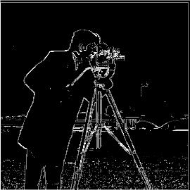
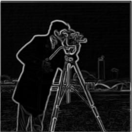
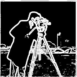
Since each post-convolution output is an image gradient, we can do √ (image_gradientx2 + image_gradienty2) to obtain the gradient magnitude. After binarizing the gradient magnitude with a threshold, the gradient magnitude will show all of the edges for the original image. Below is the original image, gradient magnitude, and binarized gradient magnitiude (threshold = 0.15):
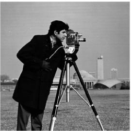
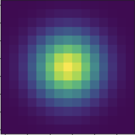
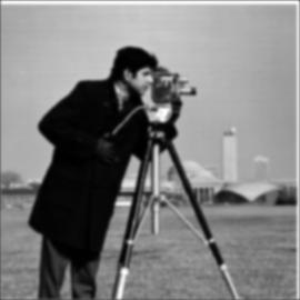
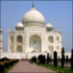
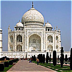
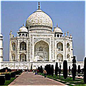
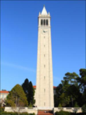
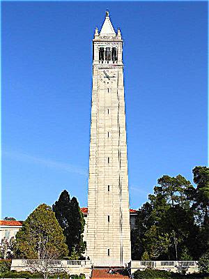
Even though the outputs from the finite difference filters are nice, they aren't quite perfect. Specifically, they can struggle for images even with a bit of noise. One way we can deal with noisy images is to use a low-pass filter, or a Gaussian blur kernel. We can create a 2D Gaussian kernel by taking the outer product with a 1D Gaussian kernel (from cv2.getGaussianKernel and its transpose. We can then obtain a blurred version of an image by convolving it with a 2D Gaussian kernel. Below are visualizations of a sample image, the 2D Gaussian kernel (window_size = 15, sigma = 5/2), and the blurred resultant sample image. We can see that the image has been blurred after the convolution with the 2D Gaussian kernel. Moreover, some of the details from the image has been lost as well (the grass, buildings in the background, camera details, etc.), which was what we were going for.
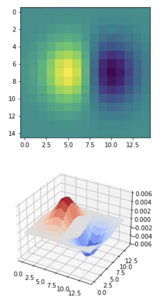
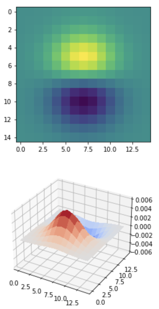
Now that we have a blurred sample image, we can find the edges on it for a more robust edge detection pipeline. However, instead of blurring the image and then convolving it twice with the finite difference filter, we can convolve the 2D Gaussian kernel with the finite difference filters, resulting in derivative of gaussian (DoG) filters. These filters are visualized below with heatmaps and 3D surface plots.
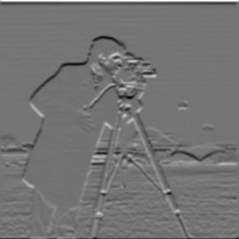
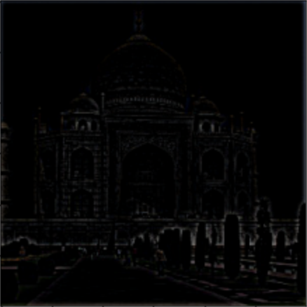
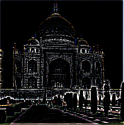
We can convolve the sample image with these DoF filters to obtain better image gradients for both the x and y dimensions (which are the first two images below). Then, we can combine them similarly to how we did in part 1.1 to obtain the gradient magnitude once again (which is the third image below). After binarizing with a threshold (0.015) again, we obtain the edges of the sample image.
When comparing the gradient magnitude found in 1.1 to the one found in 1.2, we can see that the 1.2 output is more robust and consistent. Moreover, we were able to minimize the impact of high frequencies features, such as the grass, to the overall edge detection output. Below is the gradient magnitude from 1.1 and 1.2 for comparison's sake.
Previously I showed how to blur an image and detect its edges. Now we are going to 'sharpen' an image, which means bringing out the high frequency features of the image. Thus, we want to create a high-pass filter to first extract the high frequencies. We know that the Gaussian filter acts as a low-pass filter. Therefore, the original image - blurred image = high frequencies. Shown below (from left to right) are the following: original image, blurred image, high frequencies (normal and scaled by 5) [both are clipped to fall in [0, 255]]). The gaussian filter used had a kernel_size = 15 and sigma = 5/2.
Now that we have isolated the high frequencies, we can scale them and them back to the original image to 'sharpen' the image. So sharpened_image = original_image + α * high_frequencies, where α is a parameter we can scale qualitatively. We can simplify this expression further to this: sharpened_image = original_image + α * (original_image - blurred_image). Furthermore, sharpened_image = original_image + α * (original_image - (original_image ⦻ gaussian_kernel)), where ⦻ represents the convolution operator. Now we can get sharpened_image = (1 + α) * original_image - α * (original_image ⦻ gaussian_kernel). Finally, sharpened_image = original_image ⦻ ((1 + α) * e - α *gaussian_kernel), where e is the unit impulse (identity) filter. This is the unsharp mask filter. The following images are the original image and the output of the unsharp filter for the following alpha values (1.25, 1.5, 2, 3, 4, 5, 10, 15). All of the outputs images were clipped so their values all are within the range [0, 255].


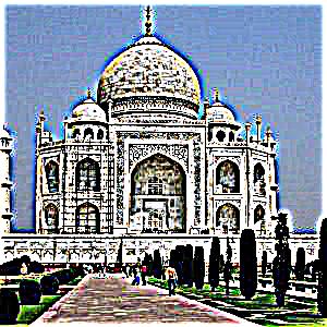
Another thing I experimented with was trying to sharpen an already sharpened image. I took a sharp image, blurred it, obtained the high frequencies, and scaled them with alpha, similar to before. I found it easier to detect the edges. However, when adding them back with alpha, I found it really easy to go above the 255 range and create weird artifacts in the image quickly (found in the sky and surround the dome). Below is the sharpened image, the sharpened image post-blurring, the detected high frequencies, and the newly sharp image output.

The following are results for sharpening for extra images. The images displayed (from left to right) are sample image, blurred image, and sharpened image.

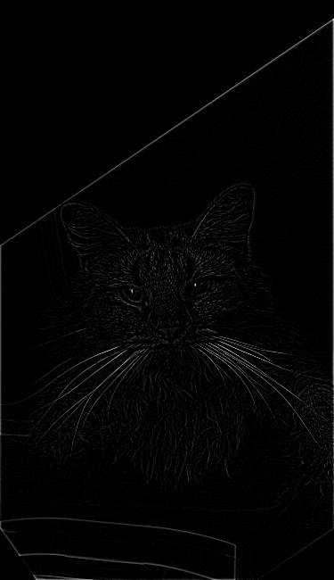
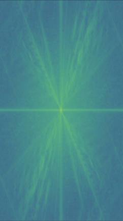
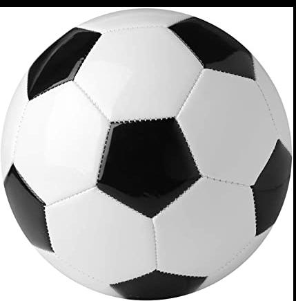
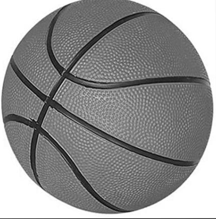
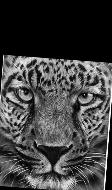
Now that we have learned how to extract low and high frequencies from an image, we can know try to combine the low frequencies of one image and the high frequencies of another image to create a 'hybrid' image. Below is an image, the image in the frequency domain, the image blurred, and the blurred image in the frqeuency domain.
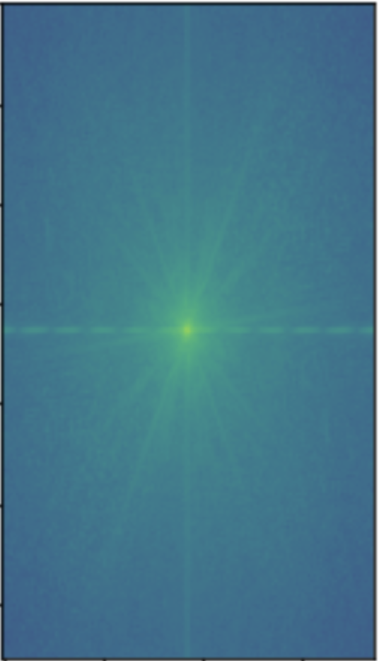

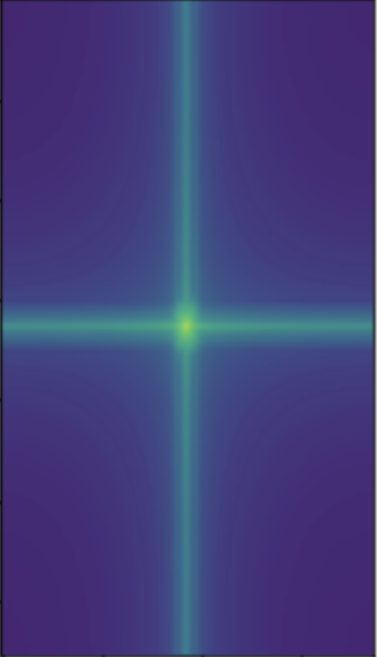
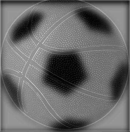
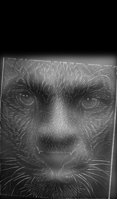
We can see from the frequency domain the only the low ones are prevalent with the blurred image. We can repeat this process for another image and obtain only it's high frequencies. Below is an image, the image in the frquency domain, the image's high frequencies, and the image's high frequencies visualized in the frqeuency domain.
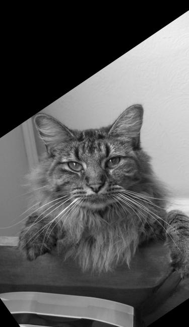
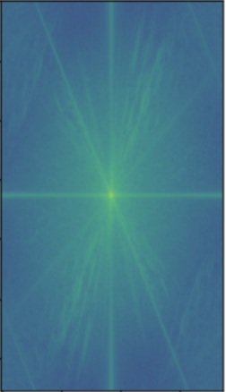
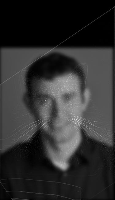
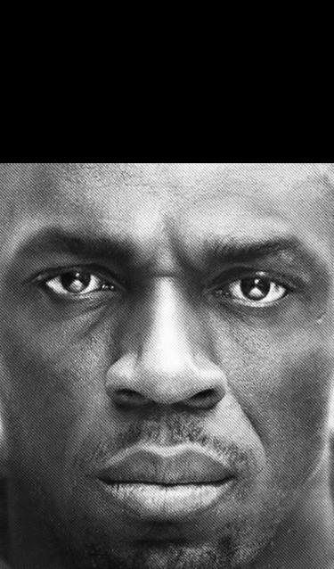
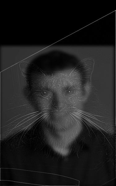
Once again we can see that the high frequencies have been isolated as the fft image gets noisier as you increase the distance to the origin. We can now average together the image_1_low_freq output and the image_2_high_freq output. The images below are the original image whose low frequencies were used, the original image whose high frequencies were used, and the hybrid result.
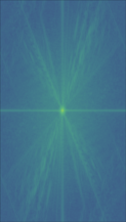
We can see that the predominant frquencies left are the low and high frequencies.
The following are results for extra hybrid image generations. The images displayed (from left to right) are image 1 for low frequency, image 2 for low frequency, and the combined hybrid image.
Here are a few failures I ran across when trying the hybrid image section!
Originally I was not normalizing the low and high frequencies at the end of the process when averaging them together causing my high frequencies to disappear from the image. Thus, I made a weighting system where I weighted the low frequencies by i and the high frequencies by 1 - i. Below is when i = 0.001 and the images were not normalized before weighted averaging:
This was when I noticed that the cat's high frequency values where in the decimal places when the low frequency image was still in the triple digits. Thus, at this point I began normalizing my images before averaging them, and my results immediately improved.
Another issue I came across was when one image could not be fit to the other (their points were too far apart to fit together). To be more specific, I was trying to click the points on a crown and on the head of a person, but since the crown was bigger than the person, the function crashed and I was not able to obtain an alignment for those two images. I wish I would've had more time to write some code to dynamically fit both images together based on the points given by the user, but I did not have the time.
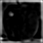
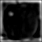
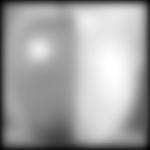
Now that we can create hybrid images, let's say we want to instead blend two images together along an image spline. The image spline will cause the boundary between the blended images to be distorted/softer. Additionally, blending these images together seperately at each band of image frequencies will allow this seam to be smoother. We will do this first by creating Gaussian and Laplacian stacks for our two images. A Gaussian stack is a stack of images that has been iteratively blurred starting from the first image in the stack, which is the sample image. In other words, for a stack of length n + 1 (since the first element is the original image), there exists n blur filters (not guaranteed to be unique) such that stack[i] * blur_filter = stack[i + 1] for i in range(n). In my implementation I kept this blur_filter to be constant throughout the stack. After calculating these Gaussian stacks for both images, we can obtain their Laplacian stacks. The process of creating a Laplacian stack is to calculate the differences between the adjacent arrays in the Gaussian stack. This will give us a stack of length n. We then append the last element of the respective image's Gaussian stack into its Laplacian stack. Now we have 2 Laplacian stacks (one for each image). We can blend these stacks together with a binary mask, which has a Gaussian stack of the same length as the Laplacian stacks for the images calculated for it. Now we can combine the 2 Laplacian stacks. The ith element in the combined stack = mask * gaussian_stack_1[i] + (1 - mask) * gaussian_stack_2. After calculating this combined stack, we sum all of the individual arrays in the stack to retrieve our blended image. Below is image 1, the mask, and image 2 used for the grayscale multi-resolution blending:
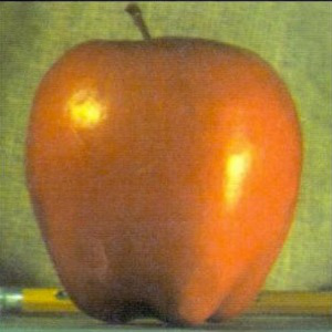

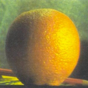
I used grayscale versions of the images for the first implementation. Each of the three rows below represent different stacks: the first row is the combined stack of the apple and the mask, the second row is the combined stack of the orange and the mask, and the third row is the final combined stack. Each column represents the level of an array within one of the stacks.

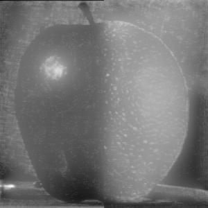
After summing over the final combined laplacian stack, we get our blended image, shown below.
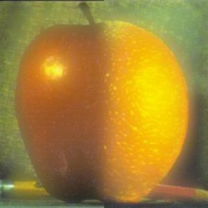
We can also generate blended images in color for doing the same blended process for each image channel. Below is the 'orapple' but in color:
Extra Color Multiresolution Blending results are shown below. The images are of the following order: original image 1, combined blended image, original image 2, binary mask.
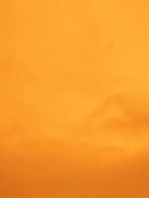
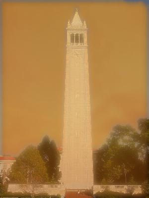
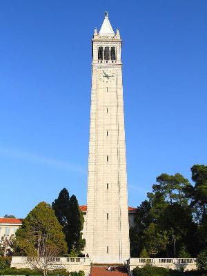
I wanted to try to combine the sky over SF during last year's wildfire season with a picture of the campanile. The binary mask was created by just filtering the blue part of the campanile image, which is why it is not completely perfect on the edges/corners.
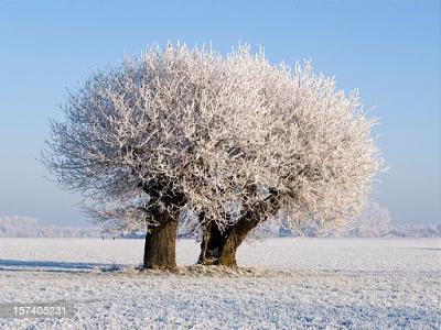
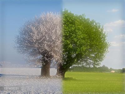
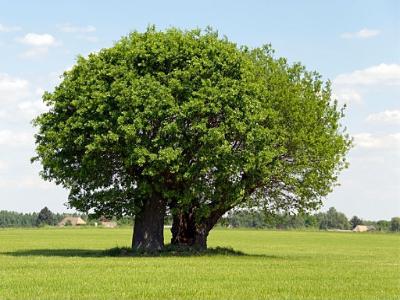
I found pictures of the same tree from different seasons. I tried to blend the winter and summer versions with the vertical mask similar to the one created for the 'orapple' (the mask is not visualized below).