---

Fun with Filters

Finite Difference Operator

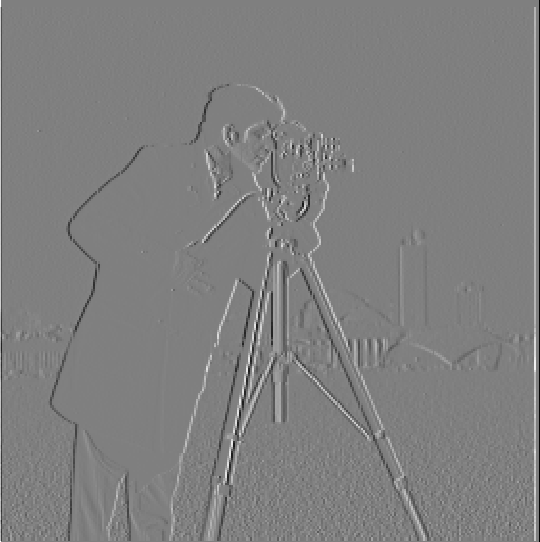
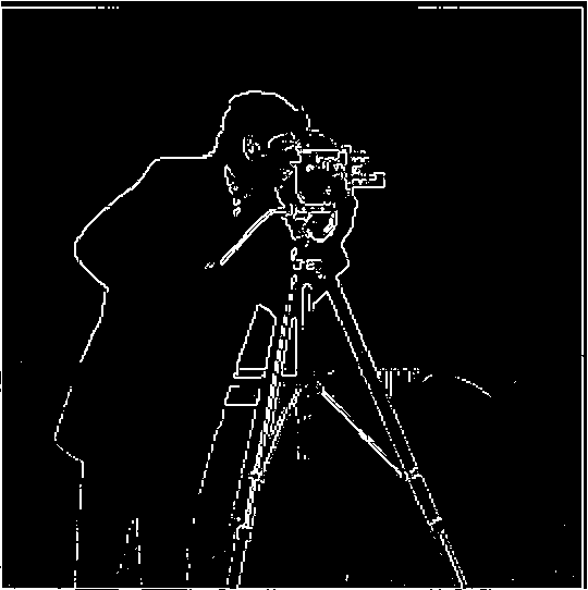
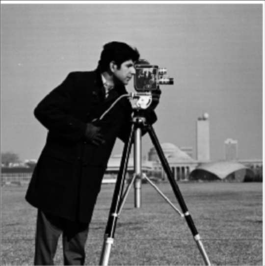
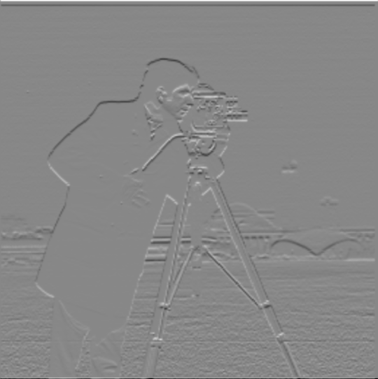
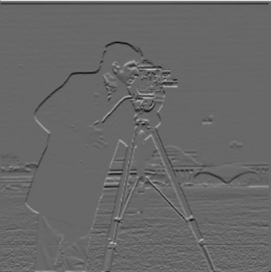
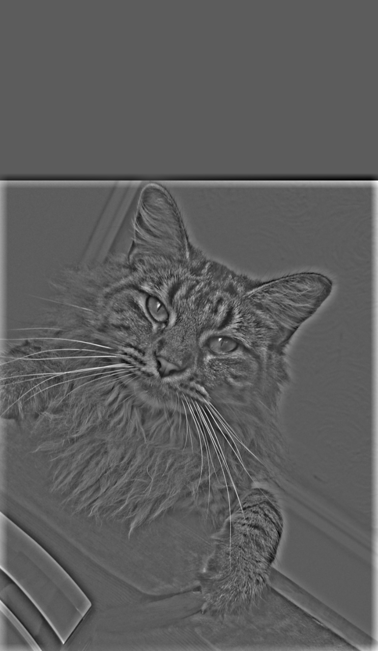
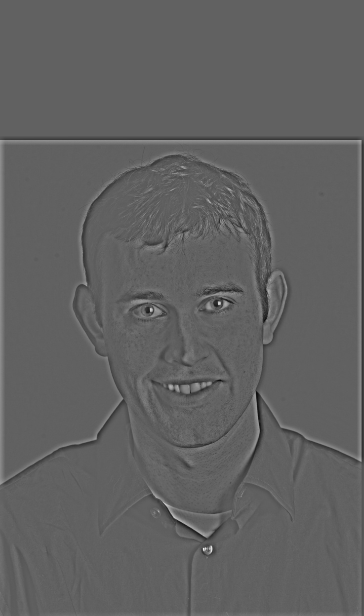
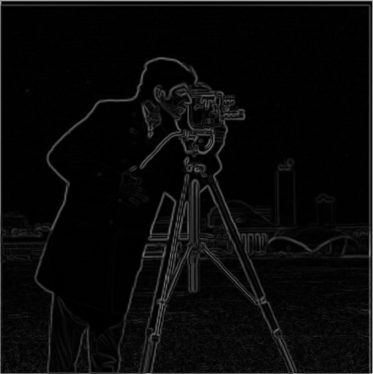
In order to find the gradient (directional change in intensity) of the cameraman, I approximated the partial derivatives of the image, through convolution with the Dx and Dy kernels. I calculated the gradient magnitude (edge strength), by squaring each of the partial derivatives of the image, then square rooting their sum. This results in a relatively decent edge-detected image, but in order to clean and suppress the noise, I binarized the image at a threshold of magnitude < 0.34.

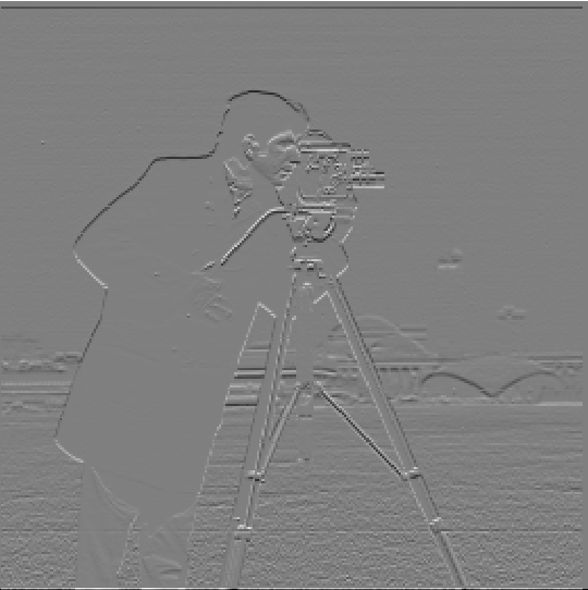
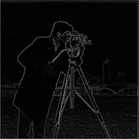
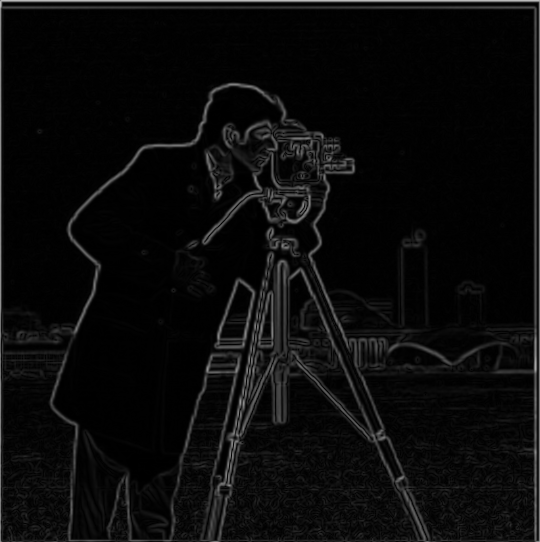
While I was able to clean/suppress noise via thresholding with the previous method, in order to create a smoother edge-detected image, I utilized the Gaussian filter.

First, I created a blurred version of the original image by convolving it with a gaussian, then repeated the previous method, with the threshold at magnitude < 0.2.

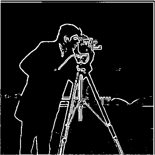
This resulted in a much smoother edge-detected image.

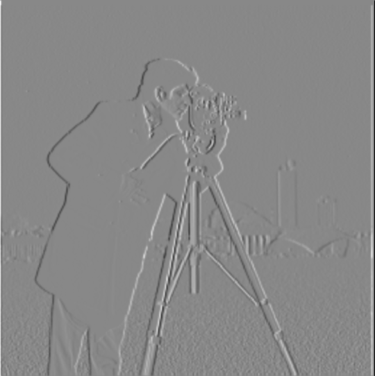
In order to reduce the number of steps/convolutions needed to find an image's smoothed edges, I created a derivative of gaussian filters by convolving the gaussian with the Dx and Dy kernels.

With these new DoG filters, I can apply them directly to the original image, without first blurring it with a gaussian convolution.

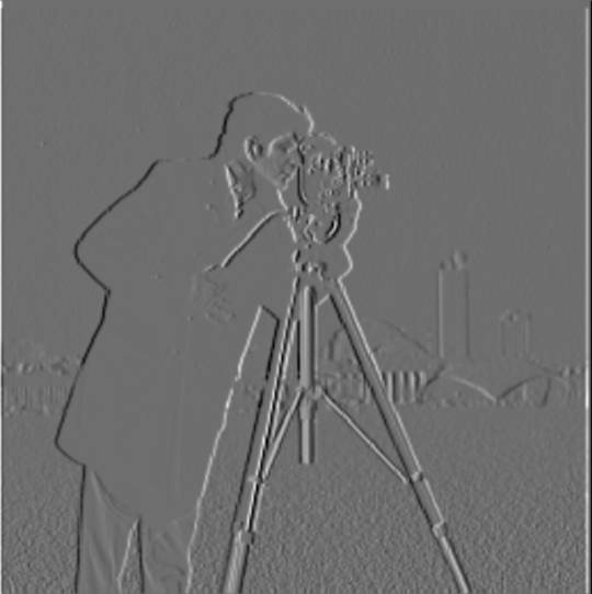
Save for floating point precision errors, the results are nearly identical.

---

Fun with Frequencies

Image Sharpening

Here, I derive the unsharp masking technique in order to sharpen images.

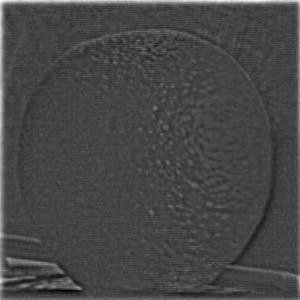
An image looks sharper if it has stronger high frequencies. So, to start, I aimed to find the high frequencies of the image, via subtraction of its low frequencies. First, I use the Gaussian filter to blur the original image (retaining only the low frequencies), then I subtracted this blurred image from the original, resulting in an isolation of its high frequencies. By adding these high frequencies (scaled by an alpha value) back to the original image, we can produce a sharper image.

From here, we can derive the unsharp mask filter, which will allow us to simplify this method and sharpen images through a single convolution operation. This series of subtractions/additions, f + alpha(f - f * g), where f is the original image, and g is the gaussian, simplifies to (1 + alpha)f - alpha(f * g), which further simplifies down to our unsharp mask filter, defined as f * ((1 + alpha)e - alpha * g), where e is the unit impulse (identify). With this newly derived unsharp mask filter, we only need to perform one convolution in order to sharpen the image for identical results.

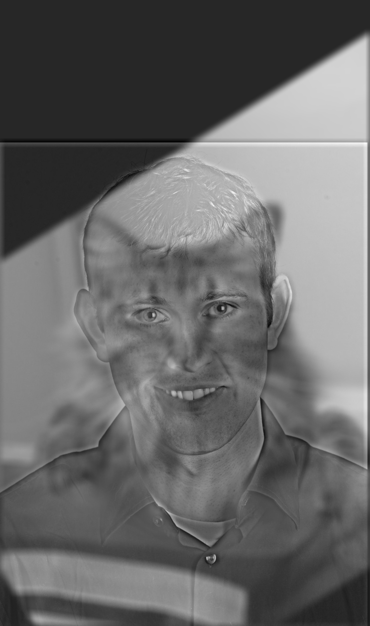
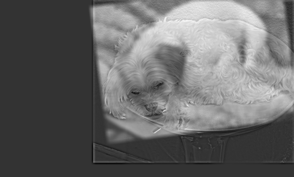
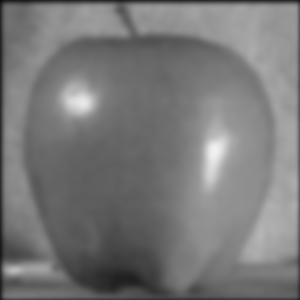
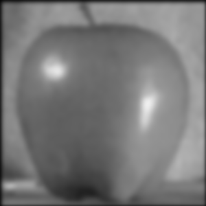
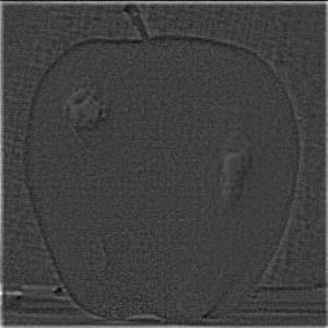
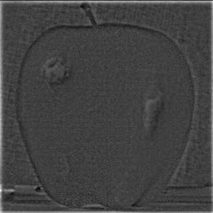
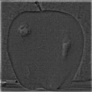
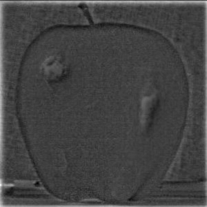
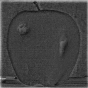
For evaluation, I blurred a sharp image, then tried to sharpen it again.

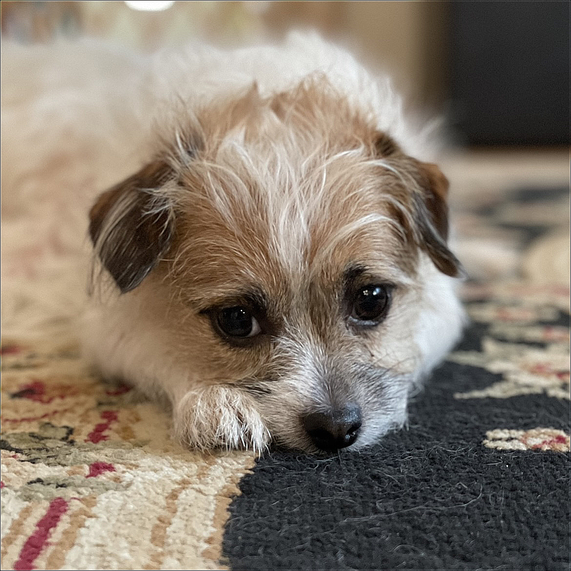
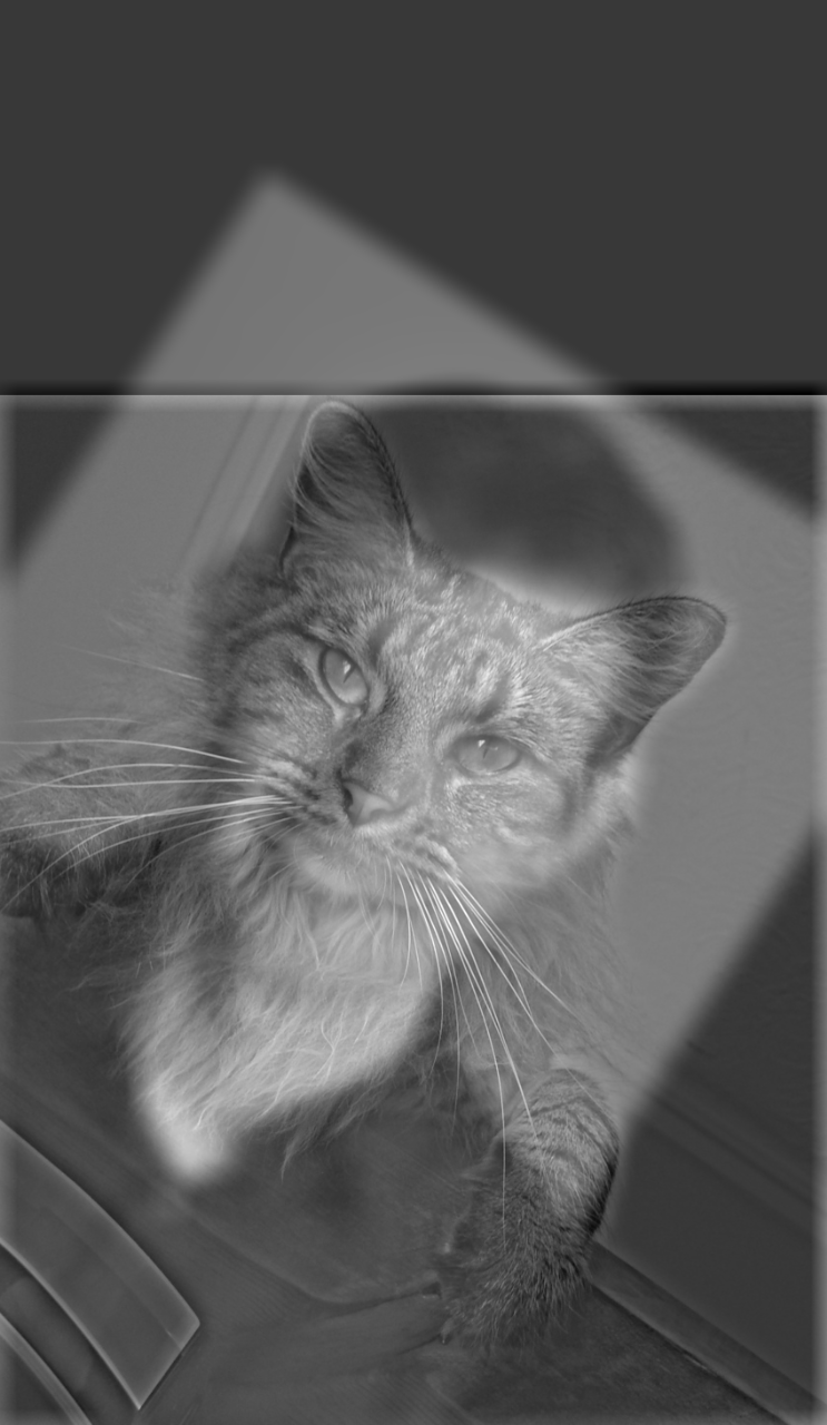
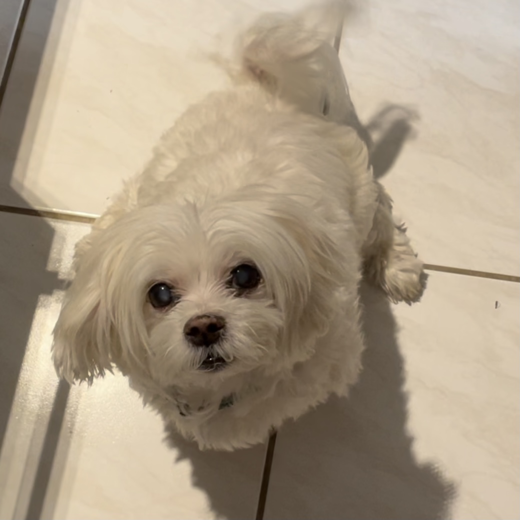
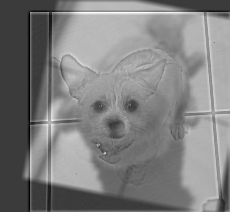
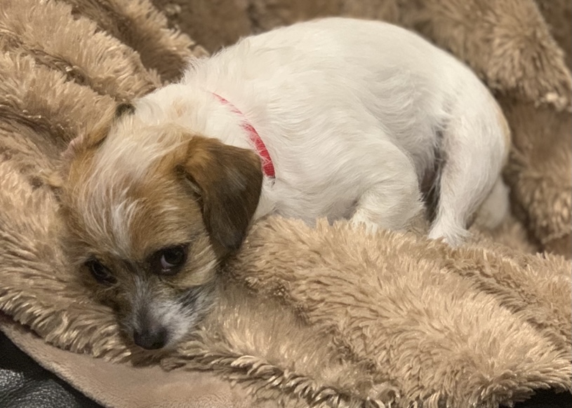
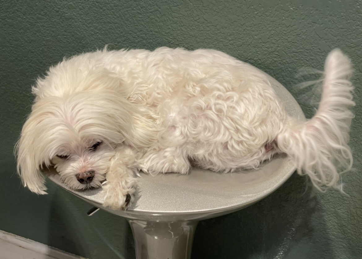
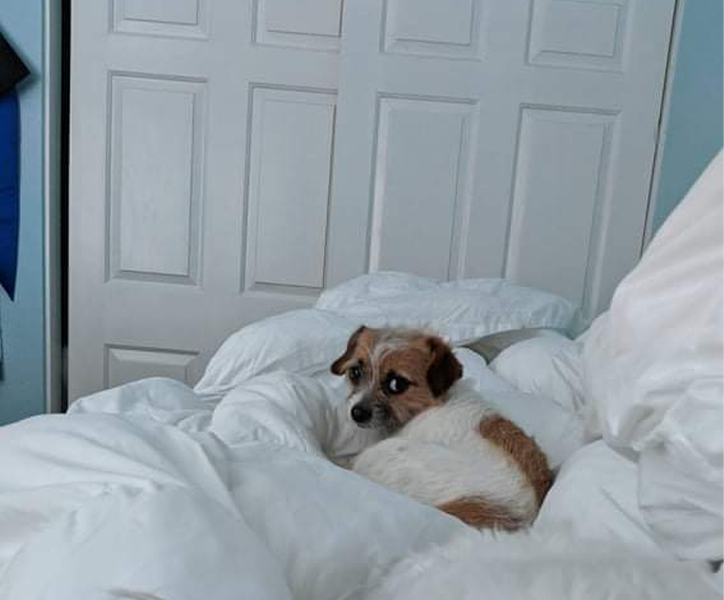
Here's another example, where I sharpen a photo of my dog, Toby.

---

Hybrid Images

Hybrid images are static images that change in interpretation as a function of the viewing distance. At close proximity, high frequencies tend to dominate perception, but at a distance, only the low frequencies are seen. In order to get a hybrid image that leads to different interpretations at different distances, I follow the approach described by Olivia, Torralba, and Schyns in their SIGGRAPH 2006 paper, by blending the high frequency portion of one image with the low frequency portion of another.

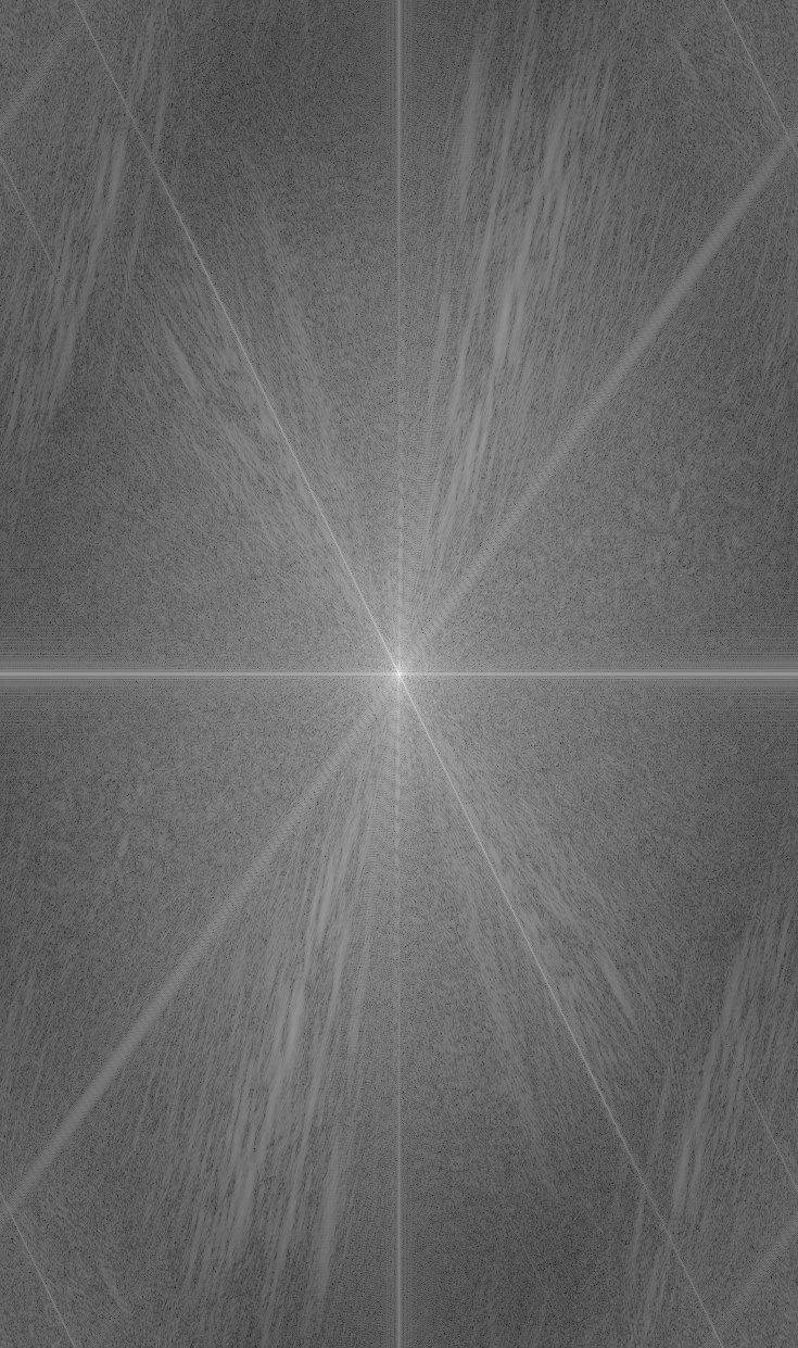
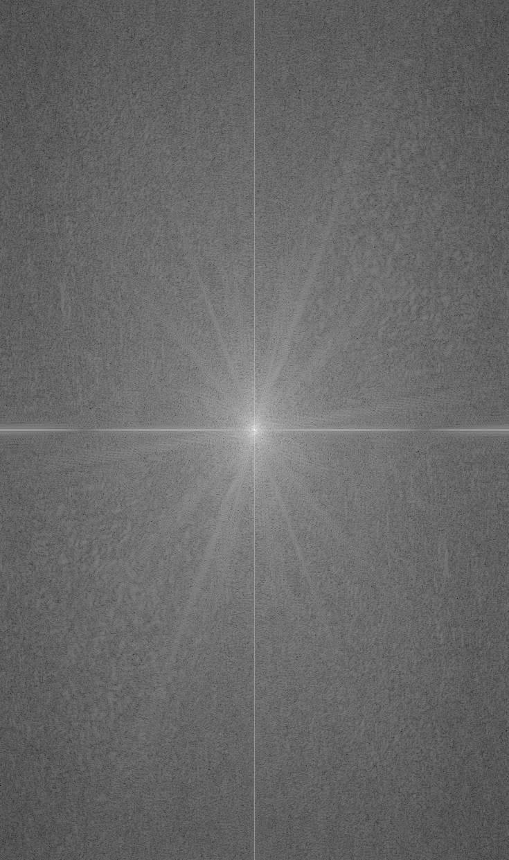
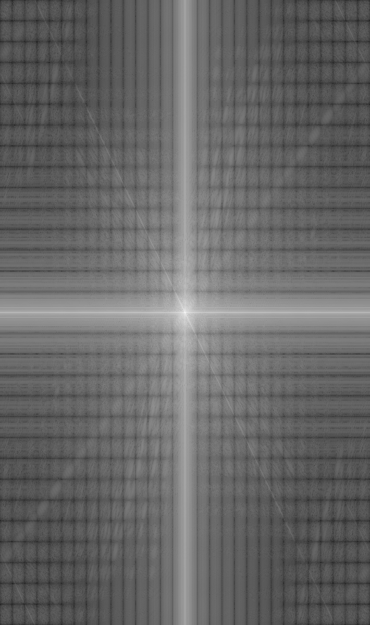
Here, I align images of Derek and Nutmeg, then combine the low-pass frequencies of Derek (found by applying a gaussian filter) with the high frequencies of Nutmeg (by subtracting its low frequencies found via the Guassian).

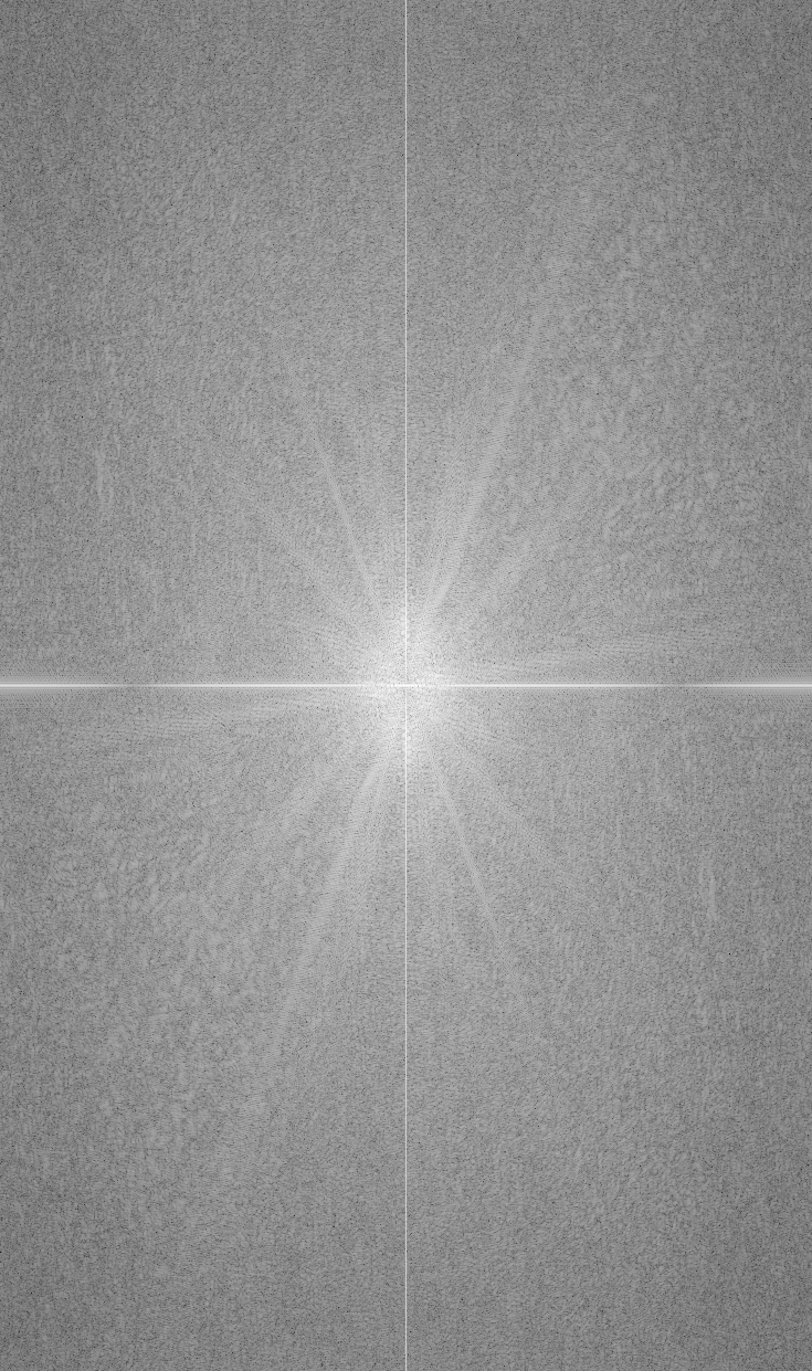
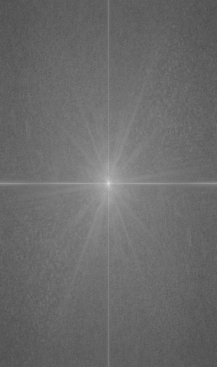
Log magnitude of Fourier transforms:

I also tried using the high frequencies of Derek with the low frequencies of Nutmeg.

More Examples

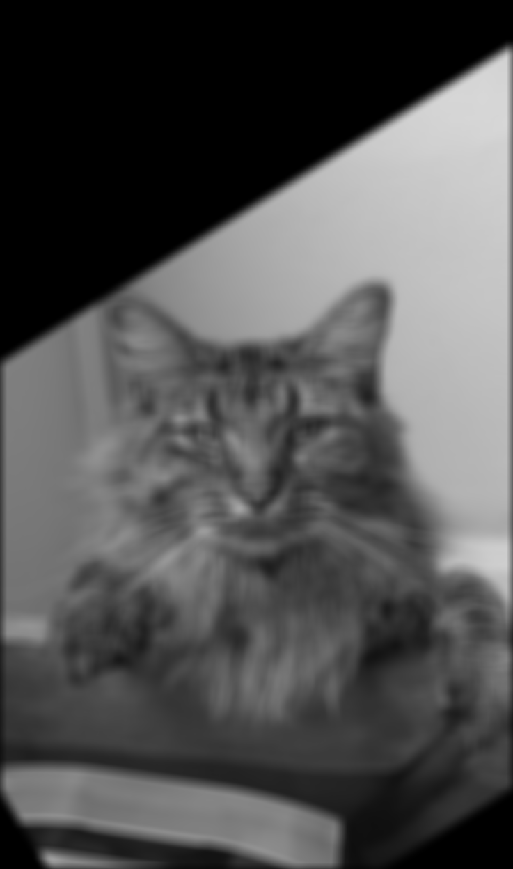
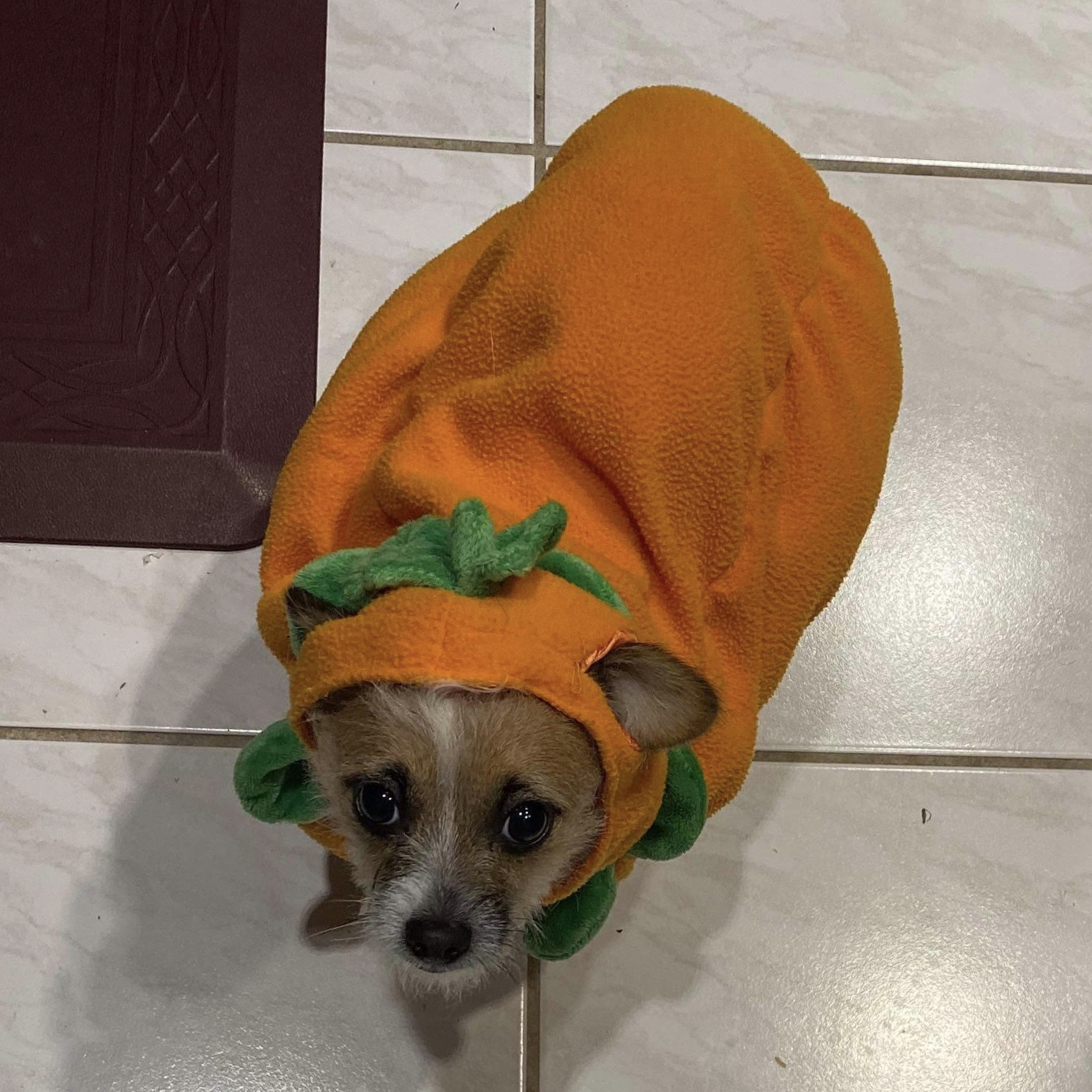
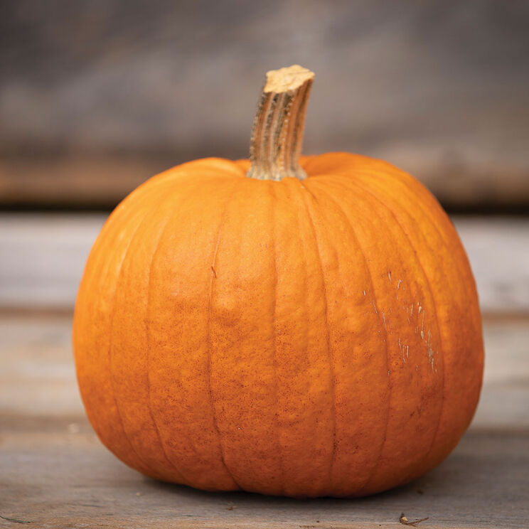
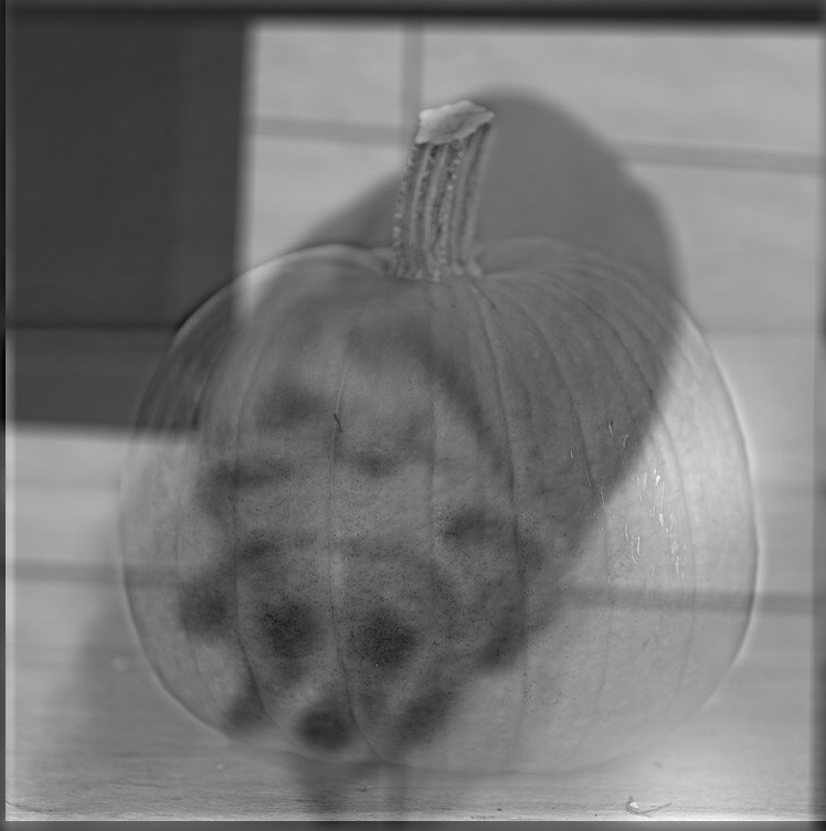
Unfortunately, this method only works well for images that have similar positioning/shapes. As much as I wanted to hybridize a picture of Toby dressed as a pumpkin with a real pumpkin, a dog shape is unfortunately pretty different from a pumpkin shape, and they don't share very many features. So, it was hard to align in a way works well.

---

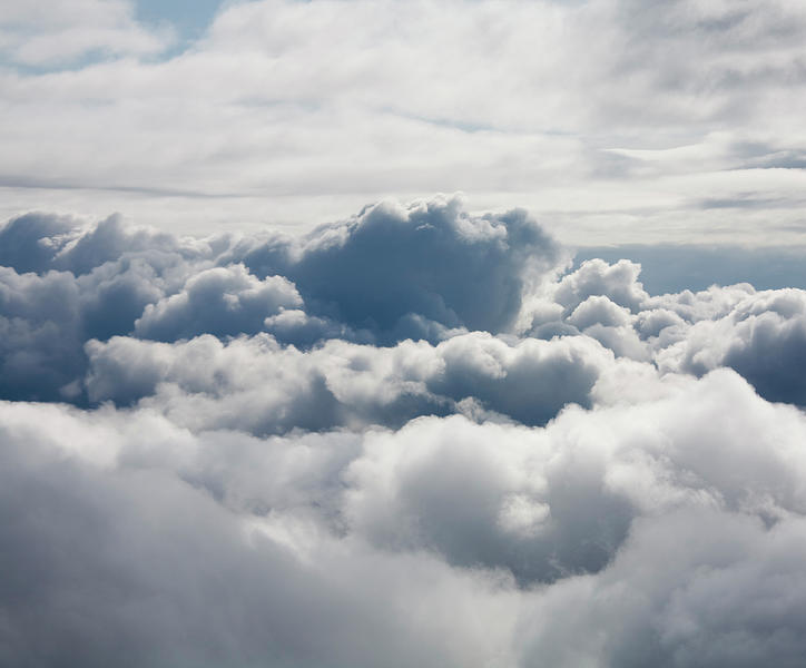
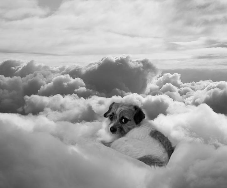
Multi-resolution blending

Here, I attempted to blend two images seamlessly using multi-resolution blending, as described in Burt and Adelson's 1983 paper. In multi-resolution blending, a gentle seam between two images is separately computed at each band of image frequencies, resulting in a much smoother seam.

To start, I created and visualized Gaussian (GA and GB, for images A and B respectively) and Laplacian stacks (LA and LB, for images A and B respectively), demonstrating the image at different levels of frequency.

Gaussian stacks (GA and GB), levels 0-5 (low to lowest frequency):

Laplacian stacks (LA and LB), levels 0-5 (high to highest frequency):

I also built a Gaussian stack (GR) for the mask. Then, using all of the created stacks, I formed a combined stack LS from LA and LB, using nodes of GR as weights:

LS = GR * LA + (1 - GR) * LB

Finally, to obtain a combined splined image, I summed each level of LS, creating the following image:

More Examples

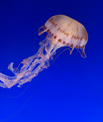
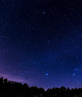
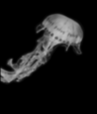
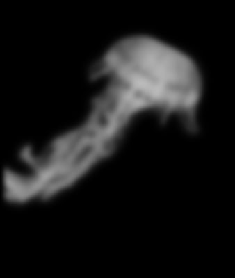
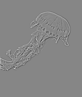
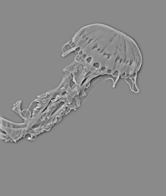
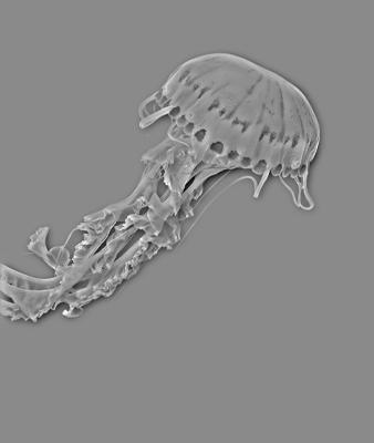
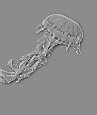
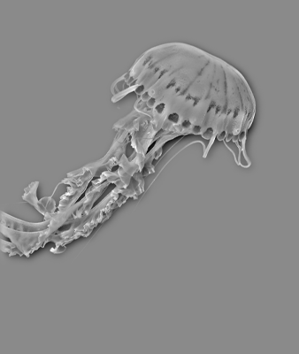
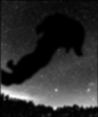
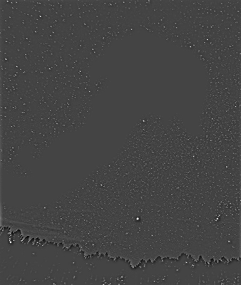
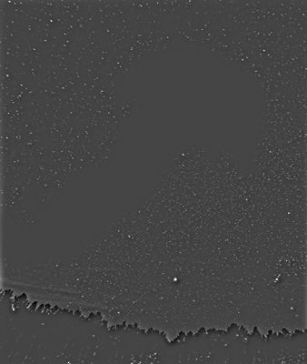
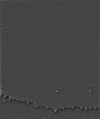
Stacks with Binary Masks applied for Giant Sky Jellyfish: