CS 194-26 Project 2: Fun With Filters and Frequencies
1.1 Finite Difference Operator
Using "gradient" filters to find edges:
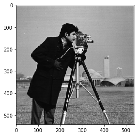
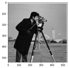
Original image :
Filters:
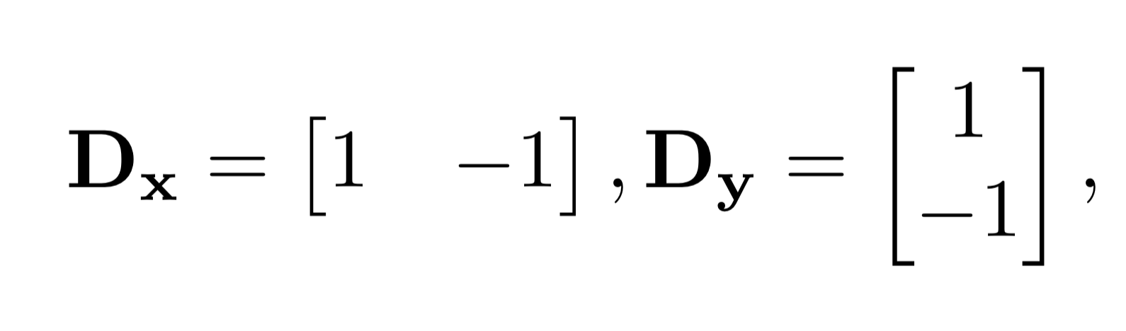
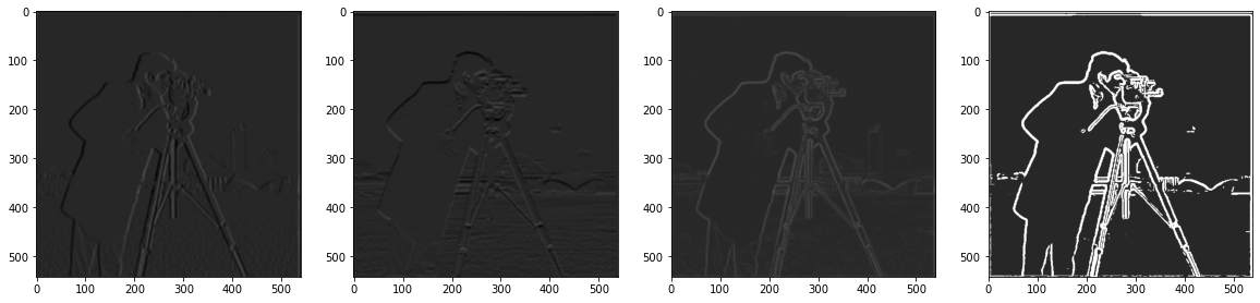
Applying and to create partial derivative images and :
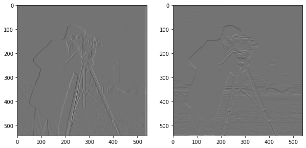
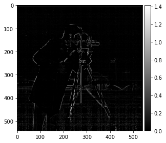
We can see that edges exist where the magnitude of the derivative is large. However, these derivative images only help us find edges for one dimension. To combine the magnitude information of both X and Y axes, we can use the magnitude of the gradient:
Which gives us the following image :
We can create a threshold image that thresholds each pixel at in the following manner:
Using we get the following image :
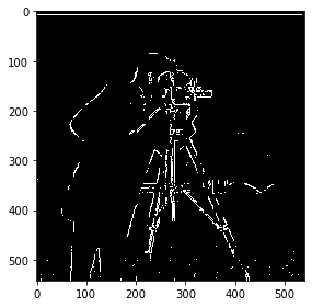
The edges are very clear, but they look broken up and don't quite cover all the important details of the man and the camera. Perhaps we can try to clean up the image first before finding the edges. We can apply a gaussian filter to blur as a low pass filter to block out noise, which usually has high frequency.
Gaussian filter with with and kernel size of 6 (from now on I will use a kernel size of for every gaussian filter):
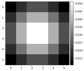
Convolving the original image with the filter (), we get the blurred image :
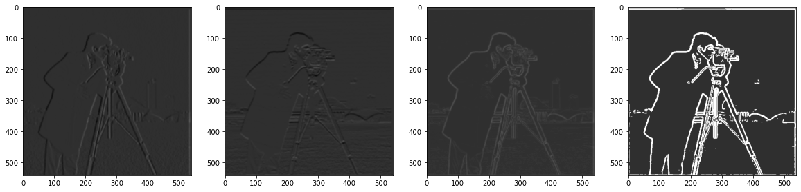
Applying the same steps (derivative filter, gradient magnitude, thresholding) on we get the following results:
Image order: and final threshold image with :
The edges look much more well-defined and the extra edges from the grass can be removed without losing details on the camera man!
1.2 Derivative of Gaussian Filter
We can combine the blurring and partial derivative steps into a single filter using the associative properties of convolutions.
Before, to get and , we had first blurred the image and then applied the derivative filter:
Using the associative property, we can rearrange the steps:
We can first apply the derivatives to the gaussian in both x and y axes and then apply these gaussian derivatives to the image to get partial derivatives of the blurred image. This way, we only need to apply a convolution to the image (which is expensive) once rather than twice.
Derivative of gaussians and , :
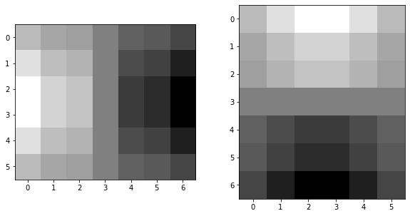
Applying and to the original image, then finding the gradient magnitude and applying a threshold (0.05), we get the exact same results as the end of 1.1!
2.1 Image Sharpening
If we capture the high frequencies of an image and add more of it back to the image, we can achieve a "sharpening" effect.
An easy way to apply a high pass filter to an image is to first apply a low-pass filter (e.g. with a gaussian filter ) and then subtract the result from the original image
We then add back to the original image:
Where can be set to a custom value. We can derive a sharpening filter by rearranging the equation:
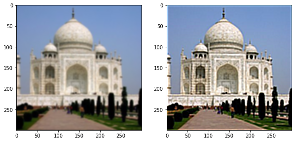
Results on taj.jpg : Original, using subtracted high pass filter, using sharpening filter.
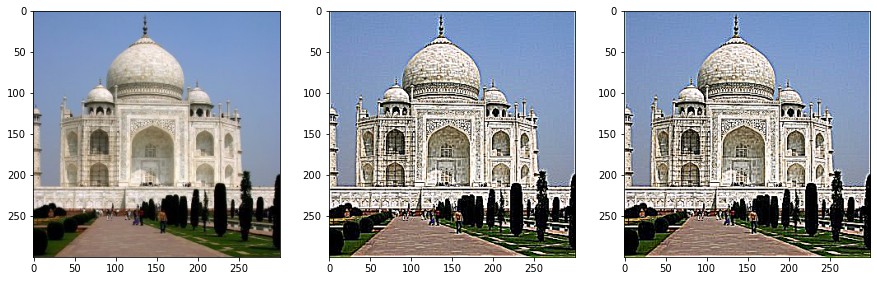
We see that the subtle details are emphasized by making the colors more extreme. If we look at the bars on the left side of the Taj Mahal, we see that the sharpened images turn the bar from a brownish gray to black, so they become more noticeable. Similarly, the shadows also become much darker.
As a test, we can apply the sharpening filter to a pre-blurred version of taj.jpg. We see the same effect where the colors become more extreme, giving the illusion that the image is less blurry, but looking closely, it is still lacking in actual resolution.
Trying the sharpening filter on other images (original, after):
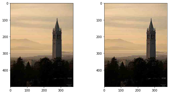
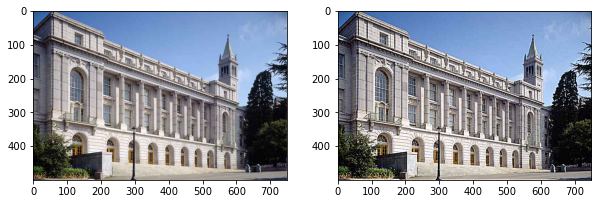
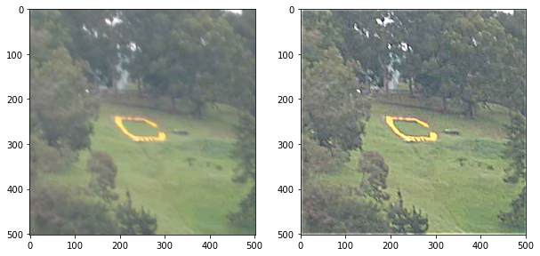
For the Campanile and Wheeler Hall, adding the sharpening filter does not add much benefit to the image, but in the case of the Big C, where the picture is blurry, applying the filter does add some benefit.
2.2 Hybrid Images
Hybrid images are images that look different at various distances. When up close, you would see one image, but when far away (i.e. meters away), you would see a complete different image. The way these images are constructed is by:
- Aligning the image (e.g. the eyes of two people)
- Applying a high pass filter for the image you want to see close up and a low pass filter on the image you want to see far away
- Averaging the filtered images together
- Normalizing the scale of the final image.
To apply a low-pass filter, we just convolve a gaussian, while for a high-pass filter, we subtract the low-passed image from the original, just like in 2.1. Note that the gaussian filter is parameterized by instead of frequency. A larger leads to a larger blur, so a low-pass filter with a lower cutoff frequency, so and frequency are inversely related.
An important detail to mention is that the cutoff frequency for the high-pass filter and the low-pass filter need to be different. In particular, . Thus, in my case . I found that is about 2x larger than for the best effect.
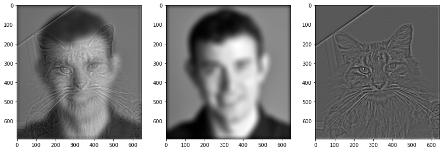
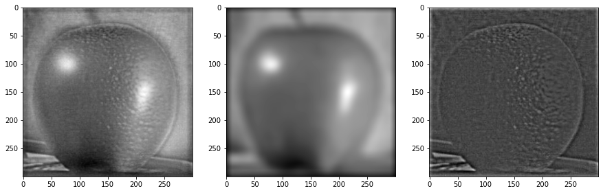
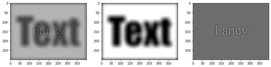
Results (hybrid image, low-passed image, high-passed image):
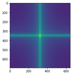
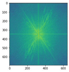
Fourier transformed derek.jpg and nutmeg.jpg
2.3 Gaussian and Laplacian Stacks
Suppose we want to blend two images together, e.g. an apple and an orange. Instead of just taking an interpolation between two images, we can do a "smarter" blend between various frequencies of the images. To create bands of frequencies we need to create a laplacian stack.
A laplacian stack can be created from a gaussian stack. At each layer, a stronger gaussian filter is applied to the image. This can be achieved by repeatedly applying a gaussian filter to the same image and saving out each iteration:
This would lead to a linear increase in of the final gaussian filter.
To make the increase in blur faster than linear, I also tried convolving the original gaussian filter with itself before applying it to the next layer, essentially doubling at each layer. I call the former way of creating the gaussian stack as linear and the latter square.
The obtain the laplacian stack, we subtract the each layer by the layer under (so the one with more blur). If we think in terms of frequency, the lower layers contain less higher frequencies, so subtracting a layer by the one below produces an image with a specific band of frequencies.
To blend images we use the following procedure:
- Create laplacian stacks of the two images
- Create a gaussian stack of the mask
- For each layer of the laplacian stack, apply the corresponding layer of the gaussian stack of the mask to the images to create a blended laplacian stack.
- Recombine the laplacian stack (just add the layers together)
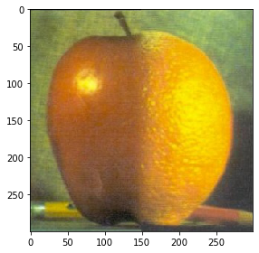
Results of the oraple:
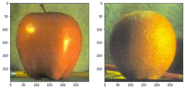
Original images:
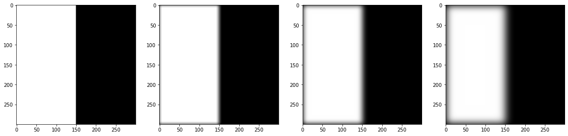
Gaussian stack of mask;
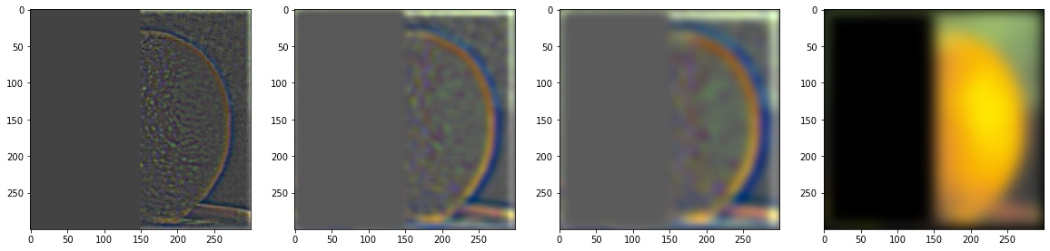
Laplacian stack of apple (with mask applied):
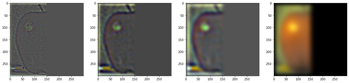
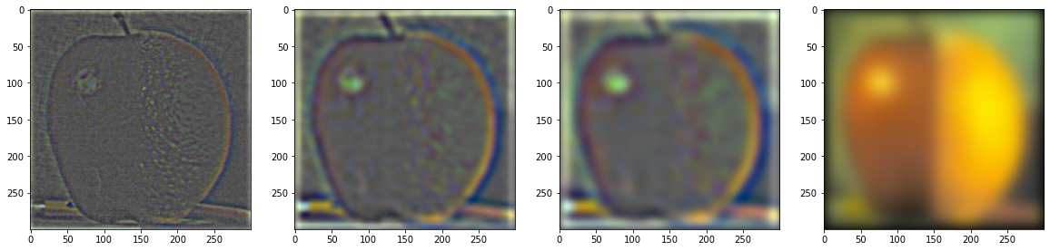
Laplacian stack of orange (with mask applied):
Blended laplacian stack:
2.4 Blending Images
Following the procedure described in 2.3, we get the resulting image for the oraple.
, filter update mode: square
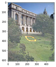
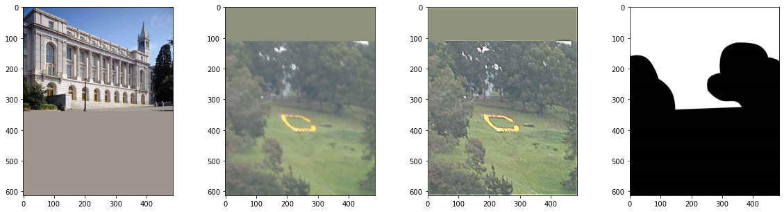
I also tried putting Wheeler hall on the Big C:
Original Wheeler Hall image, original Big C, sharpened Big C (used for blending), mask
Blended image, , 4 layers, square filter updates