CS194-26: Intro to Computer Vision and Computational Photography, Fall 2021
Project 2: Fun with Filters and Frequencies!
Angela Chen
Part 1: Fun with Filters
Part 1.1: Finite Difference Operator
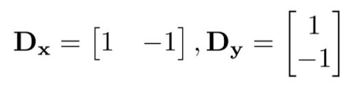
The finite difference operators to be used as the filters in the x and y directions.
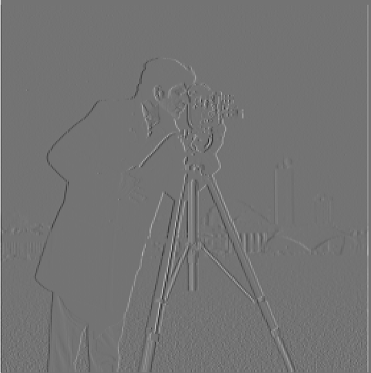
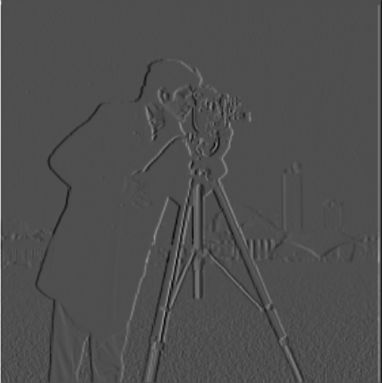
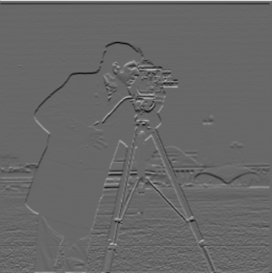
dimg/dx. img * D_x. Partial derivative in x of the cameraman image.
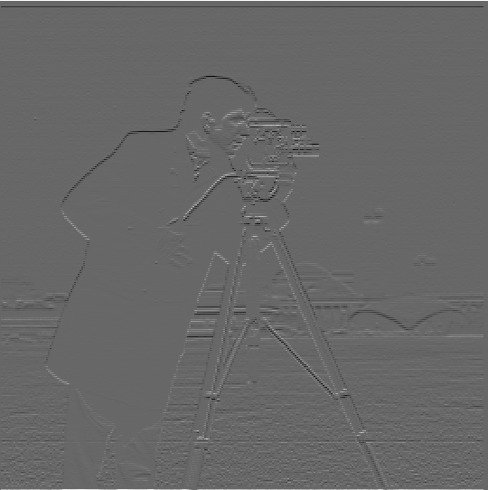
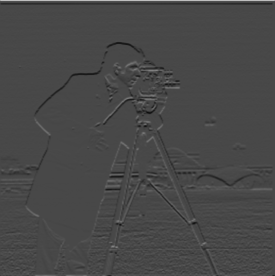
dimg/dy. img * D_y. Partial derivative in y of the cameraman image.
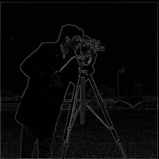
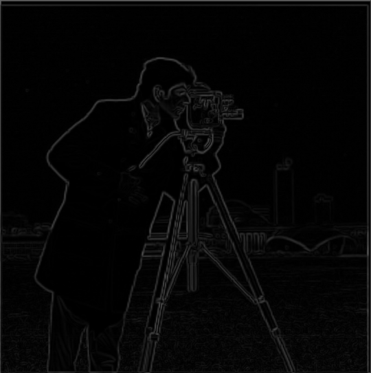
Gradient magnitude image of cameraman.Gradient magnitude = sqrt((dimg/dx)**2 + (dimg/dy)**2).
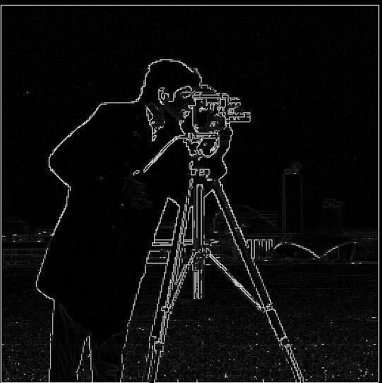
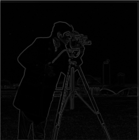
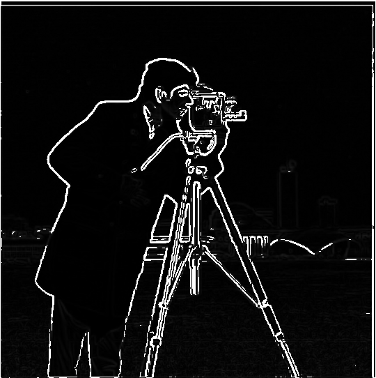
Binarized gradient magnitude cameraman image, emphasizing edges.threshold = 0.25. All values above threshold were set to 1.0.
Part 1.2: Derivative of Gaussian (DoG) Filter
For my Gaussian filter, I chose a kernel size of 5 and a sigma value of 1.
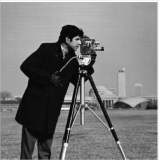
blurred_cameraman. Blurred version of cameraman by convolving with a Gaussian.
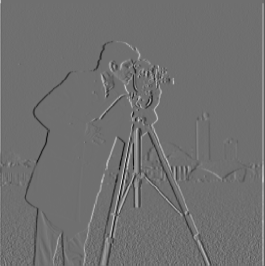
Partial derivative in x of cameraman (no blurring).
Partial derivative in x of blurred_cameraman.
Partial derivative in y of cameraman (no blurring).
Partial derivative in y of blurred_cameraman.
The edges of the partial derivative images on blurred_cameraman look much stronger and smoother with
fewer visual artifiacts than the edges of the partial derivative images on cameraman without blurring.
Gradient magnitude image of blurred_cameraman.
Binarized gradient magnitude image of blurred_cameraman, emphasizing edges.threshold = 0.1. All values above threshold were set to 1.0.
Here, the edges of the edge image are much bolder, and there's less noise in the bottom of the image.
Now, I first convolve my Gaussian with D_x and D_y, respectively, to get DoG filters.
Gaussian convolved with D_x.
Gaussian convolved with D_y.
Original cameraman convoled with DoG in x.
Original cameraman convoled with DoG in y.
Gradient magnitude image of cameraman using DoG filters.
Binarized gradient magnitude image of cameraman using DoG filters, emphasizing edges.threshold = 0.1. All values above threshold were set to 1.0.
I can see that the gradient magnitude image and edge image using DoG filters are the same as
the gradient magnitude image and edge image using a blurred version of cameraman convoled with the Gaussian.
Part 2: Fun with Frequencies!
Part 2.1: Image "Sharpening"
A simple way to "sharpen" a blurry image is to add more high frequencies to the original image.
To get the high frequencies of an image, you can convolve the original image with a Gaussian filter,
which is a low pass filter that retains only the low frequencies, to obtain a blurry version of the original imgage.
Then, you can subtract the blurred version from the original image to get the high frequencies of the image.
From there, you can scale the high frequencies by any constant alpha and add them to the original image to get a more "sharpened" image.
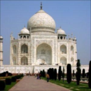
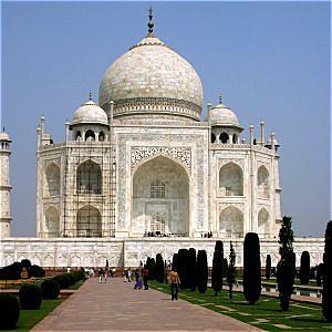
The original taj.jpg. Kinda blurry.
blurred_taj. Blurred version of taj by convolving with a Gaussian with kernel size = 5 and sigma = 1.
High frequencies of taj. taj_high_freq = taj - blurred_taj.
You can do all this sharpening in a single convolution operation, which is called the unsharp mask filter.
unsharp mask filter = f * ((1 + alpha) * e - alpha * g), where e = unit impulse (identity) filter,
f = image, g = Gaussian. I used this unsharp mask filter to get the following "sharpened" images using various values of alpha.
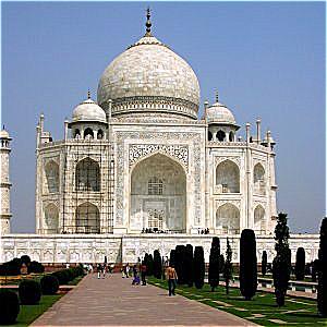
"Sharpened" taj with alpha = 1.
"Sharpened" taj with alpha = 2.
"Sharpened" taj with alpha = 3.
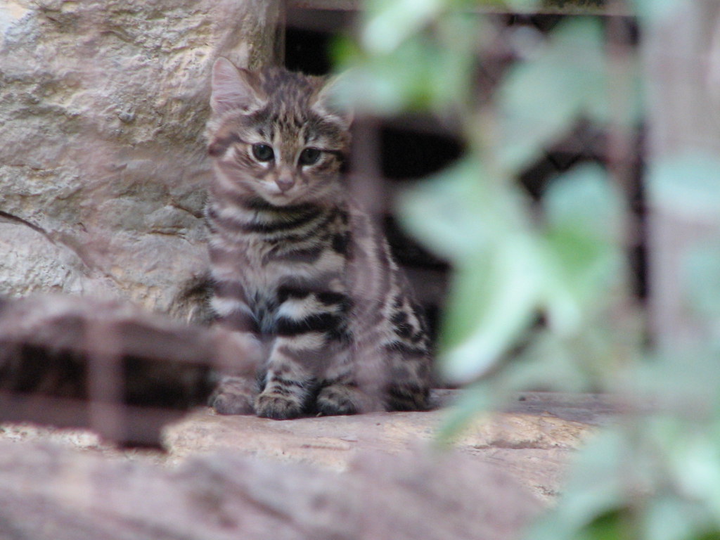
cat.jpg.
"Sharpened" cat with alpha = 7, using kernel size = 5 and sigma = 1.
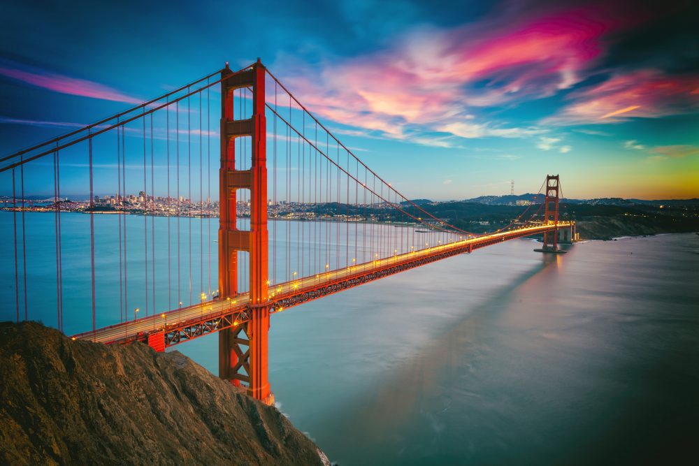
Already pretty sharp golden_gate.jpg.
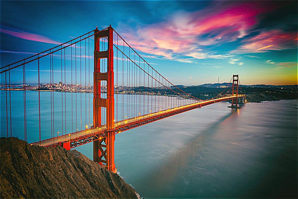
Blurred golden_gate.
"Sharpened" golden_gate with alpha = 1.
Part 2.2: Hybrid Images
To create a hybrid image of two images, you can extract the low frequencies of one image by convolving with a Gaussian filter and
the high frequencies of the other image by subtracting the blurred version of this image convolved with the Gaussian from the original image.
Then to get the hybrid image, you just add the blurred version of the one image and the high frequencies of the other image together.
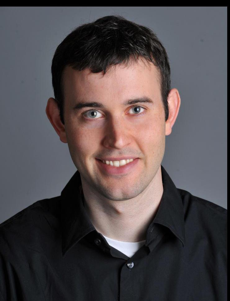
Aligned and cropped derek.jpg.
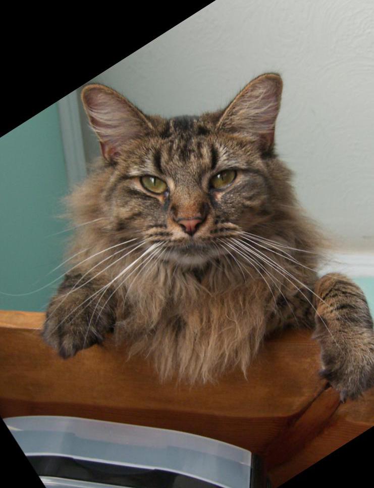
Aligned and cropped nutmeg.jpg.
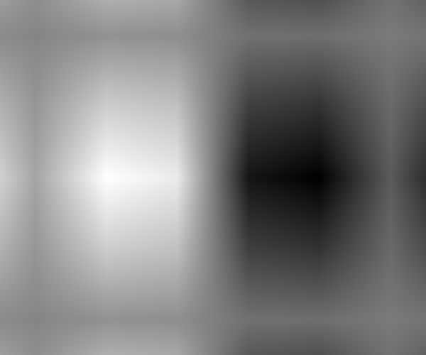
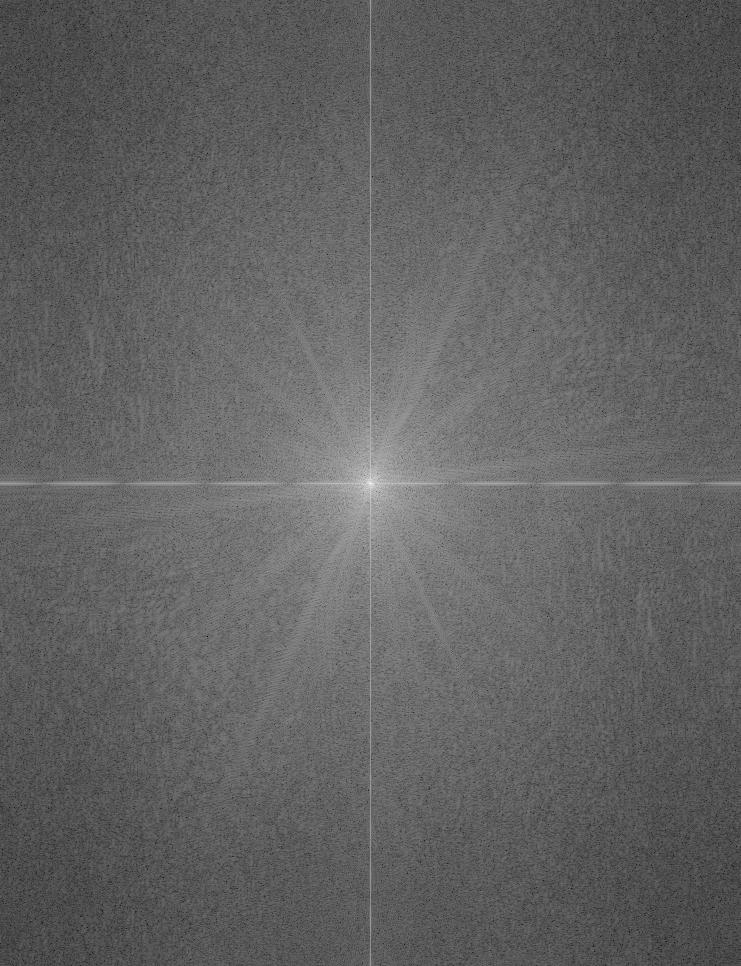
Fourier analysis of derek.
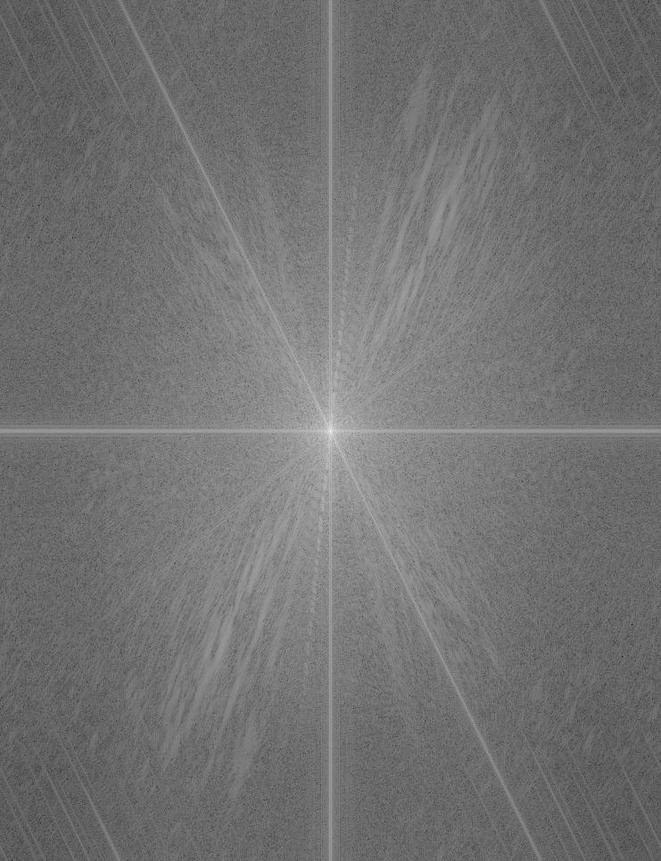
Fourier analysis of nutmeg.
blurred_derek with kernel size = 33 and sigma = 13.
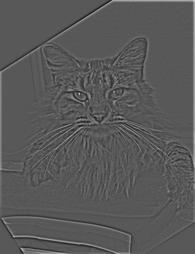
nutmeg_high_freq with kernel size = 19 and sigma = 13.
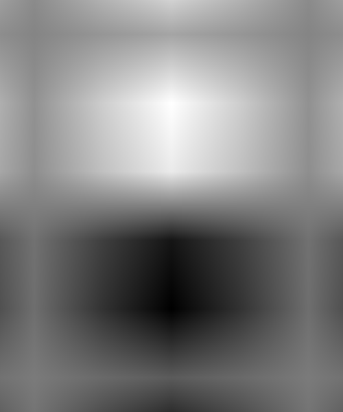
Fourier analysis of blurred_derek.
Fourier analysis of nutmeg_high_freq.
hybrid_derek_nutmeg. Hybrid image of derek and nutmeg.
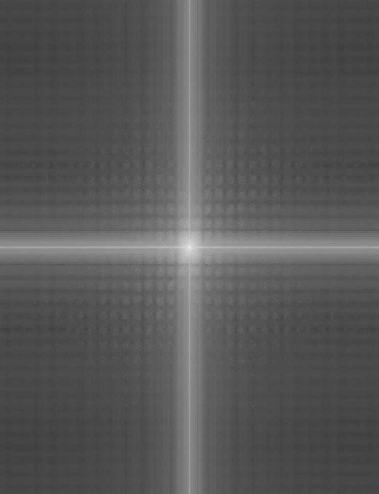
Fourier analysis of hybrid_derek_nutmeg.
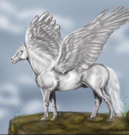
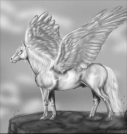
Aligned and cropped pegasus.jpg.
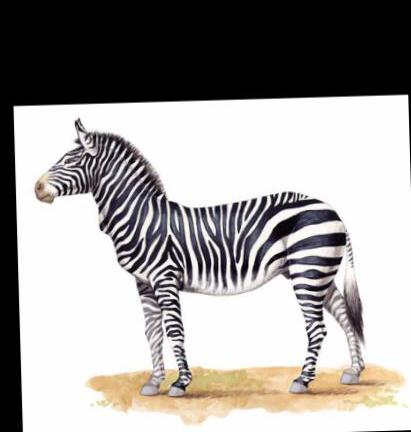
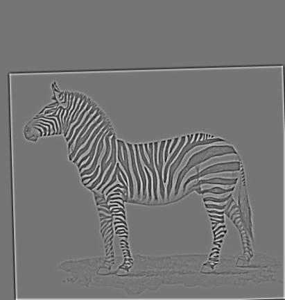
Aligned and cropped zebra.jpg.
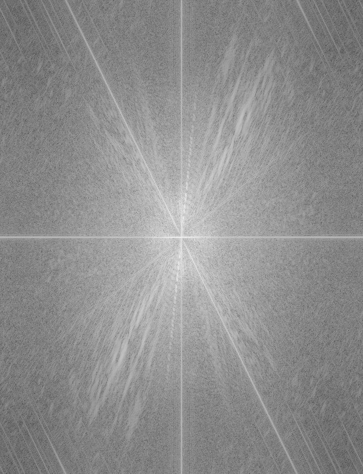
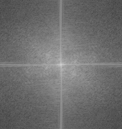
Fourier analysis of pegasus.
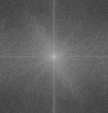
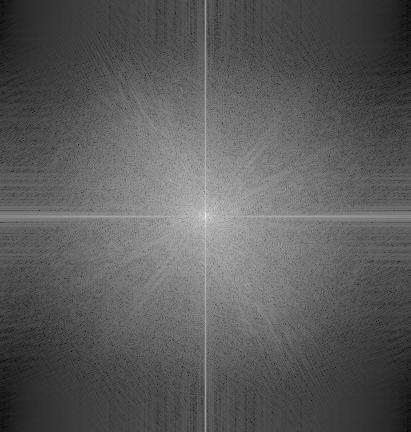
Fourier analysis of zebra.
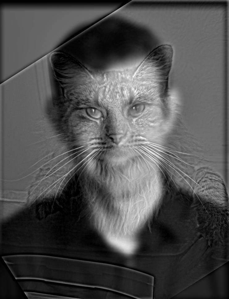
blurred_pegasus with kernel size = 5 and sigma = 1.
zebra_high_freq with kernel size = 7 and sigma = 3.
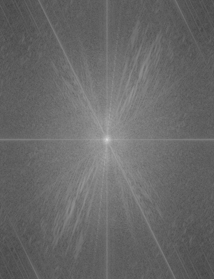
Fourier analysis of blurred_pegasus.
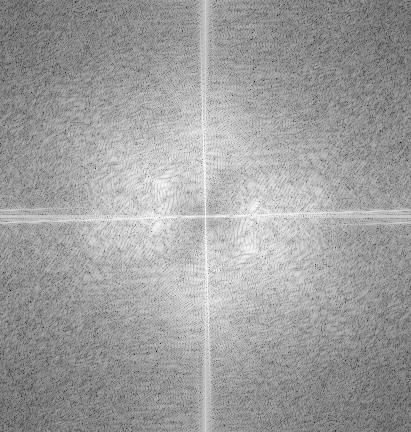
Fourier analysis of zebra_high_freq.
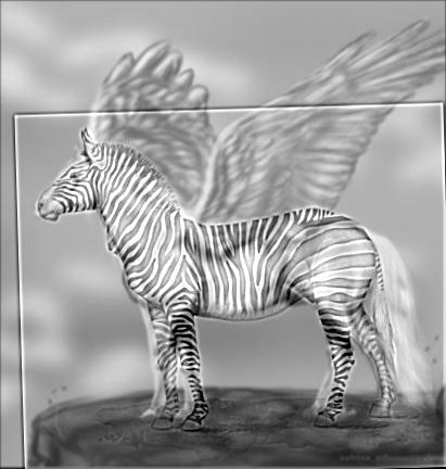
hybrid_pegasus_zebra. Hybrid image of pegasus and zebra.
Fourier analysis of hybrid_pegasus_zebra.
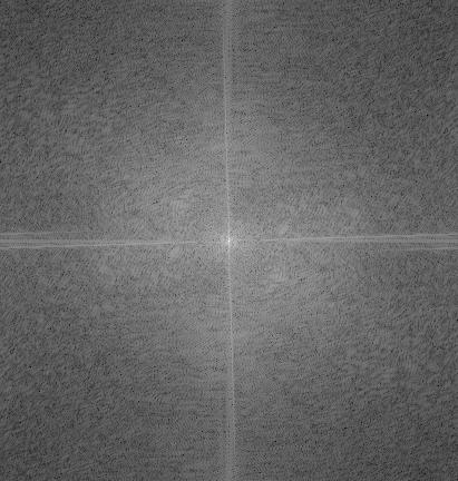
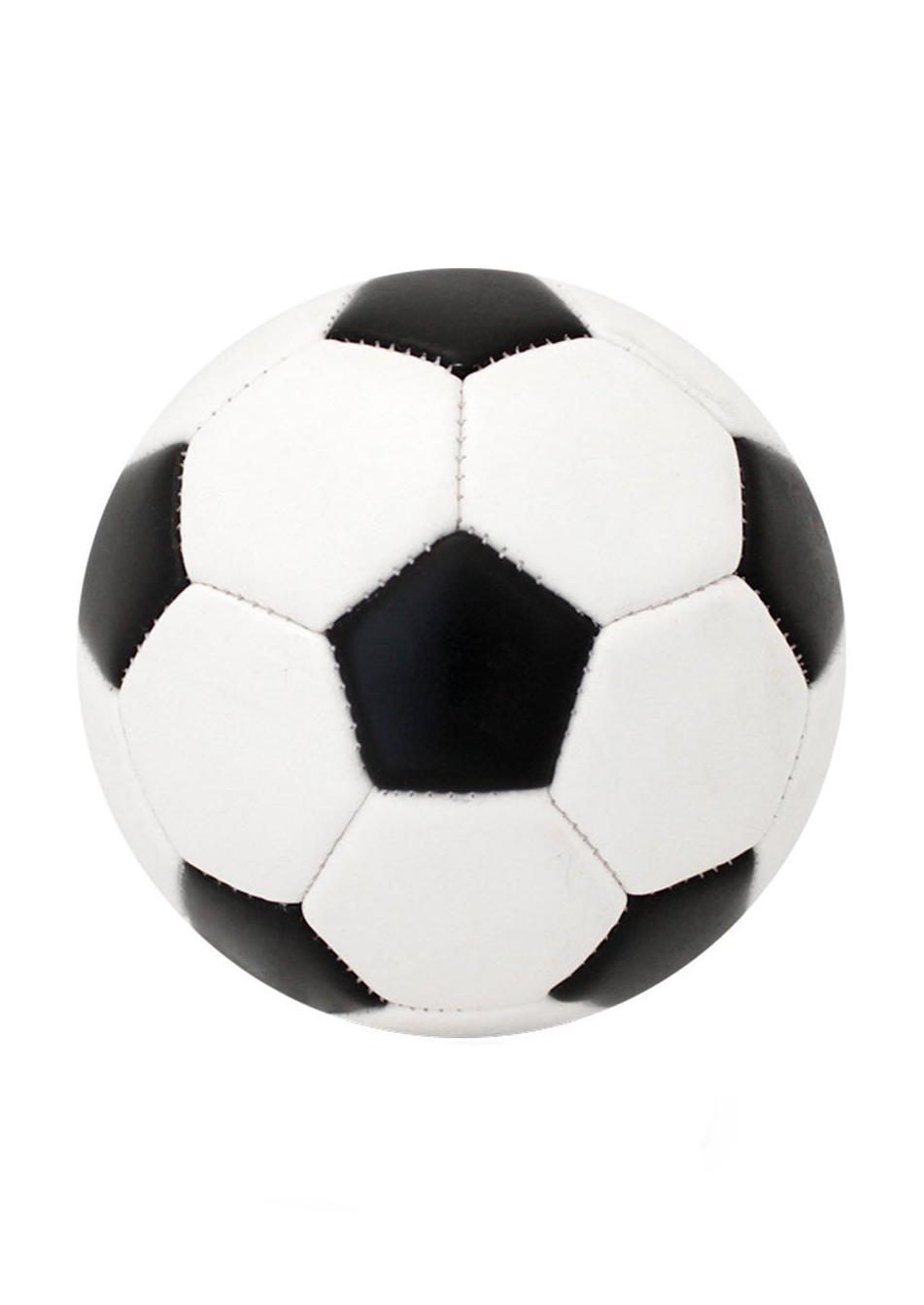
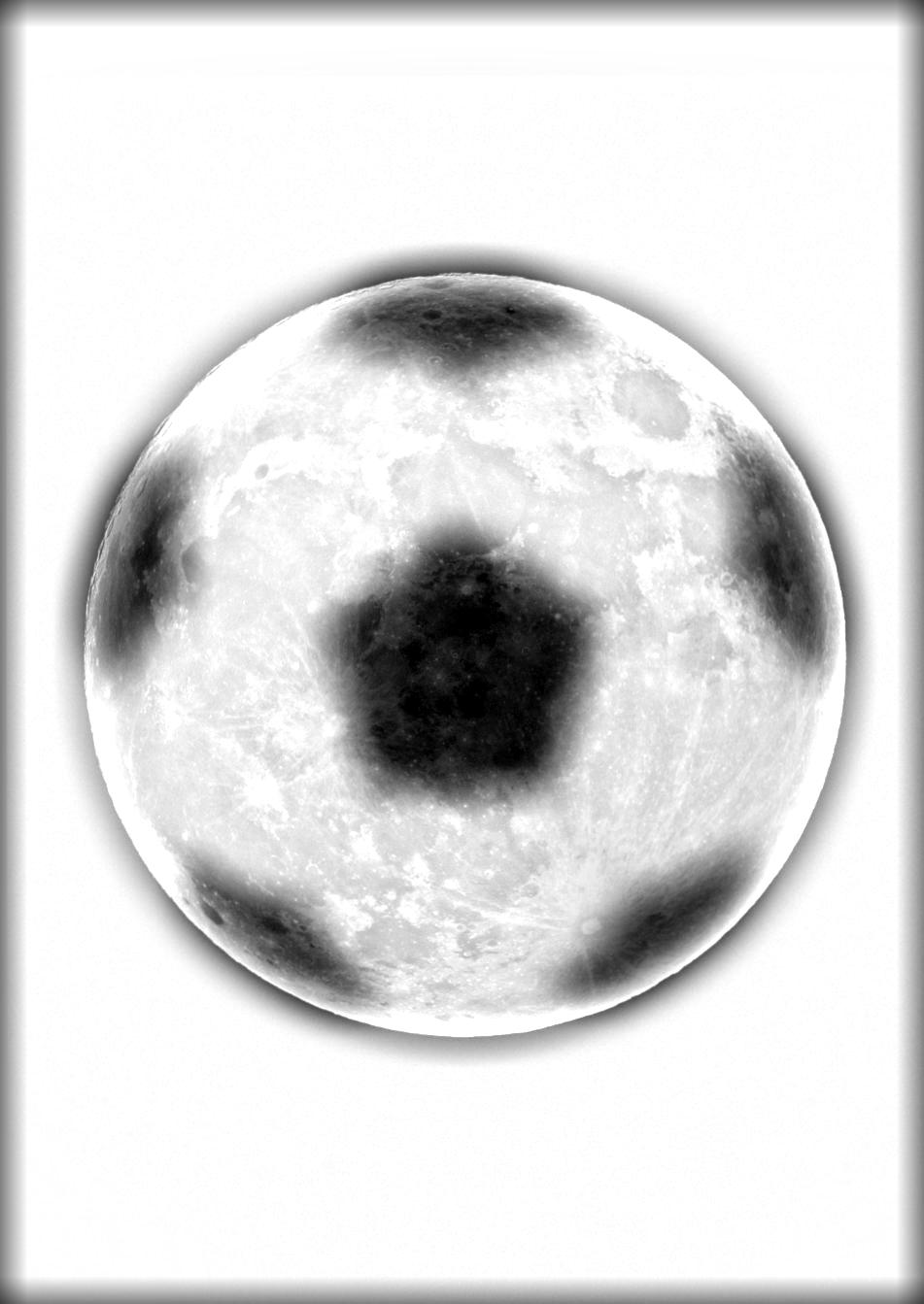
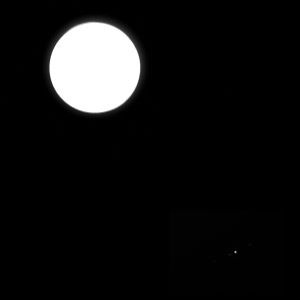
Aligned soccer_ball.jpg.
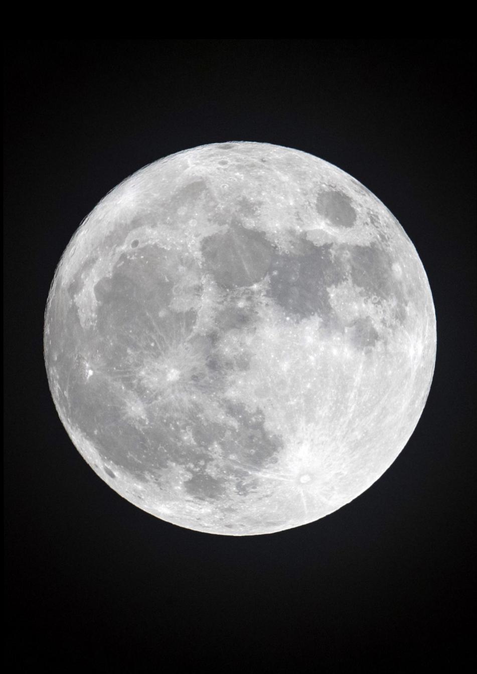
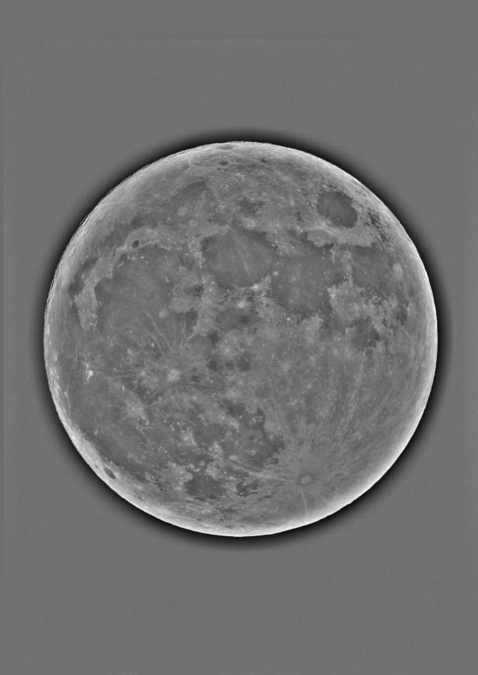
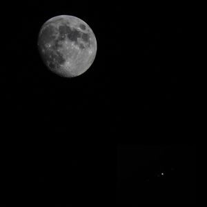
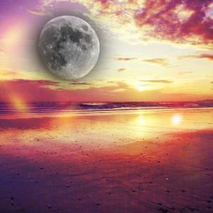
Aligned moon.jpg.
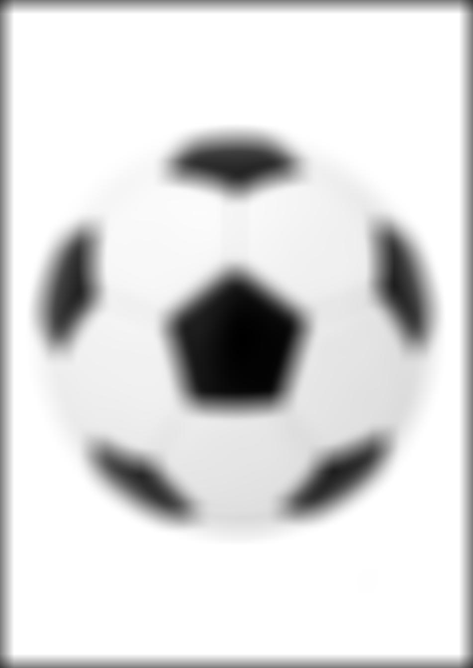
blurred_soccer_ball with kernel size = 57 and sigma = 55.
moon_high_freq with kernel size = 67 and sigma = 65.
hybrid_soccer_ball_moon. Hybrid image of soccer_ball and moon.
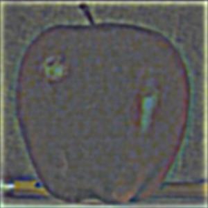
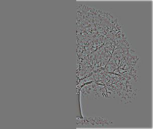
Part 2.3: Gaussian and Laplacian Stacks
To create a Gaussian stack, I stored the original image in the stack first. Then I convolved the previous image with a Gaussian to get the image for the next level.
For each level, I doubled sigma.
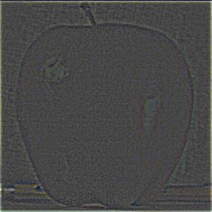
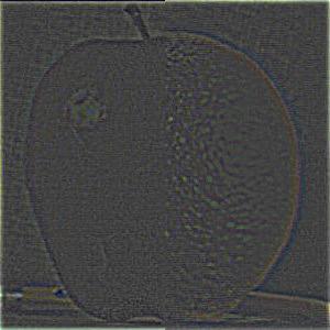
To create a Laplacian stack for an image, I first computed the Gaussian stack for the image. For each level i of the Laplacian stack, the Laplacian image
is the level i+1 image of the Gaussian stack subtracted from the level i image of the Gaussian stack. For the last level of the Laplacian stack, the Laplacian
image is equal to the last level image of the Gaussian stack.
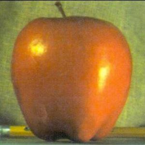
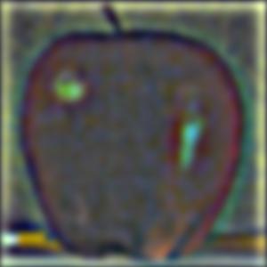
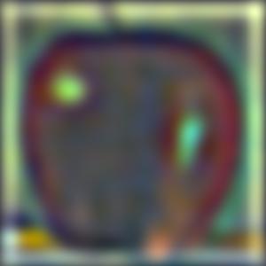
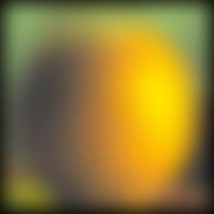
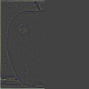
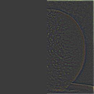
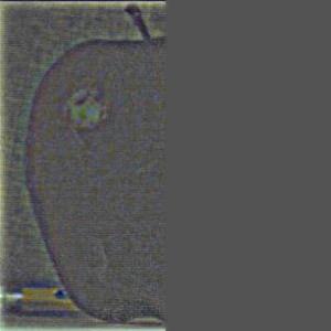
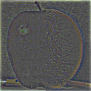
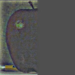
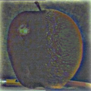
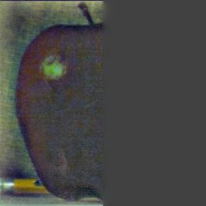
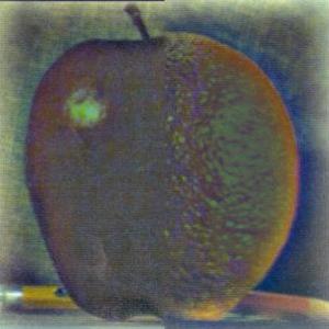
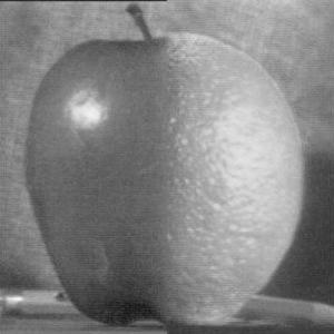
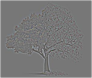
Left column is Gaussian stack for apple. Right column is Laplacian stack for apple, and I normalized the images.
Used kernel size = 45, sigma = 2, and 5 levels.
level 0
level 1
level 2
level 3
level 4
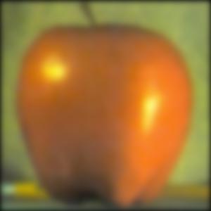
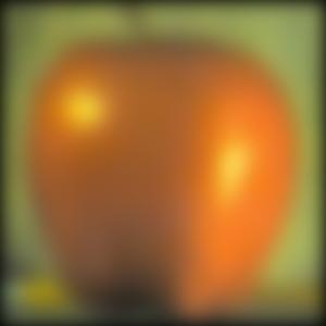
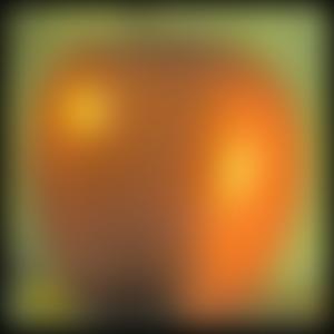
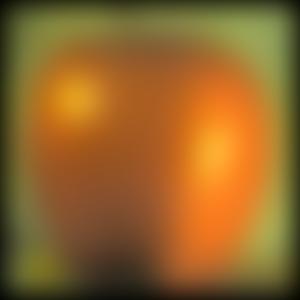
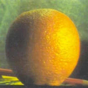
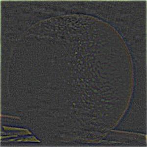
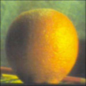
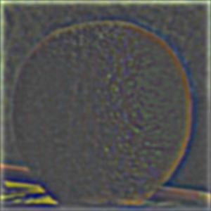
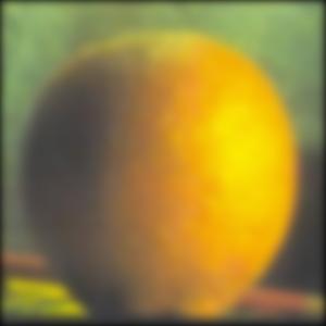
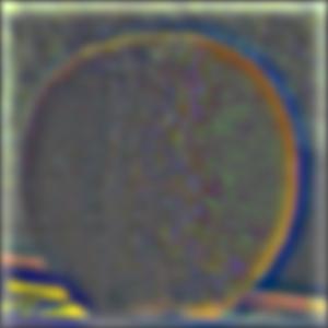
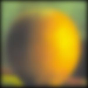
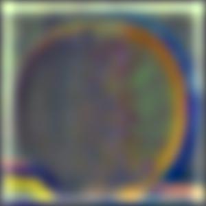
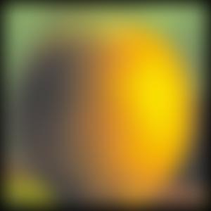
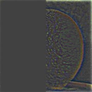
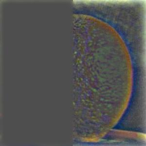
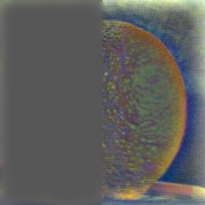
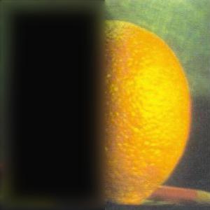
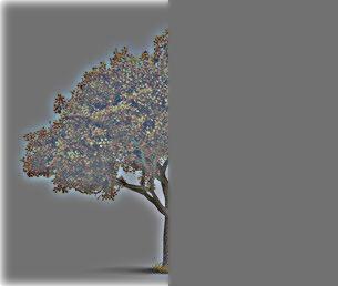
Left column is Gaussian stack for orange. Right column is Laplacian stack for orange, and I normalized the images.
Used kernel size = 45, sigma = 2, and 5 levels.
level 0
level 1
level 2
level 3
level 4
level 0
level 1
level 2
level 3
level 4
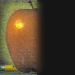
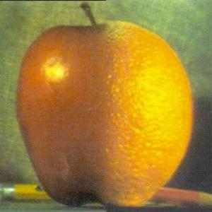
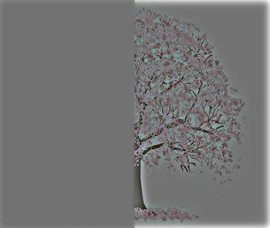
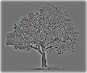
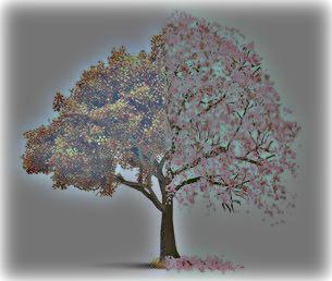
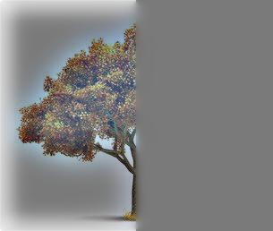
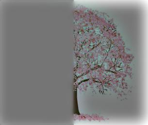
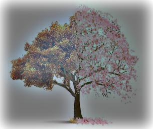
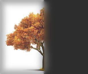
Part 2.4: Multiresolution Blending
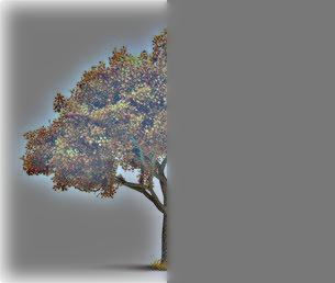
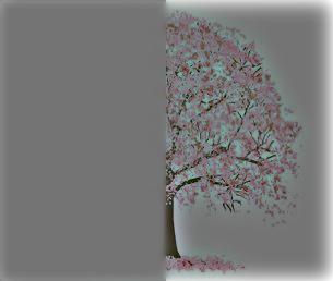
To blend two images, left_image and right_image, using a mask, I first created left_image_laplacian_stack and right_image_laplacian_stack.
I then created the Gaussian stack for the mask, mask_gaussian_stack. For every level i, I calculated
left_blended_image = mask_gaussian_stack[i] * left_image_laplacian_stack[i] and right_blended_image = (1 - mask_gaussian_stack[i]) * right_image_laplacian_stack[i].
With the final blended_image being an accumulative sum of blended_image += left_blended_image + right_blended_image.
Oraple using kernel size = 45, sigma = 2, and 5 levels.