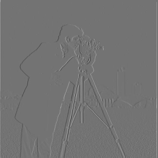
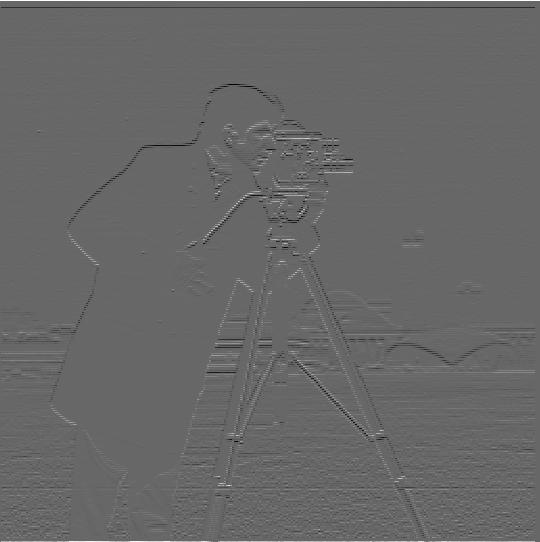
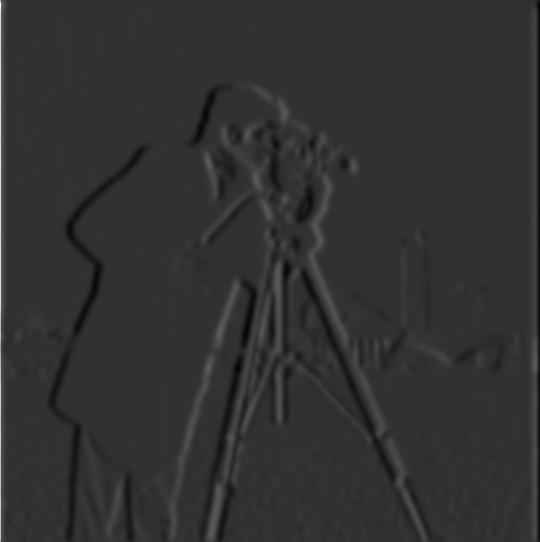
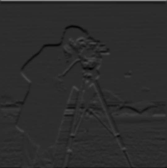
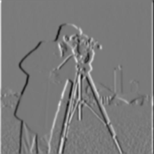
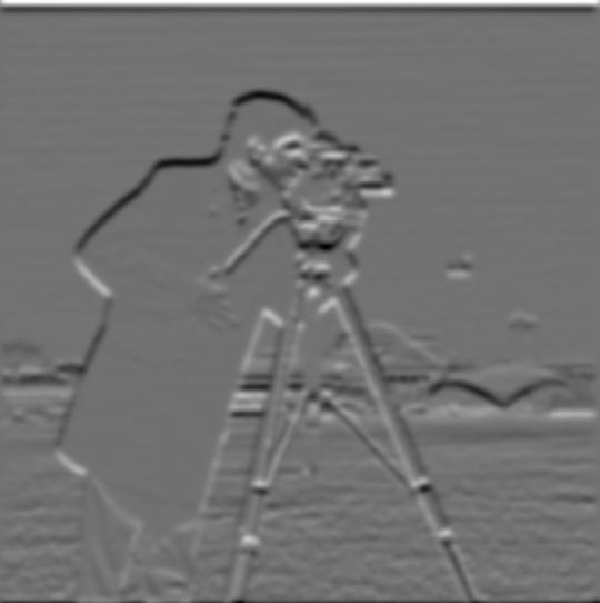
For this part we are building the Finite Difference Operator. This is done by taking the partial derivate of the x axis and y axis.
To the x axis, we will convolve the image with [1,-1]. While for the y axis, we will convolve the image with [[1],[-1]].
The is the image with regards to the derivative of x axisThe is the image with regards to the derivative of y axis
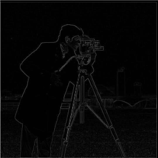
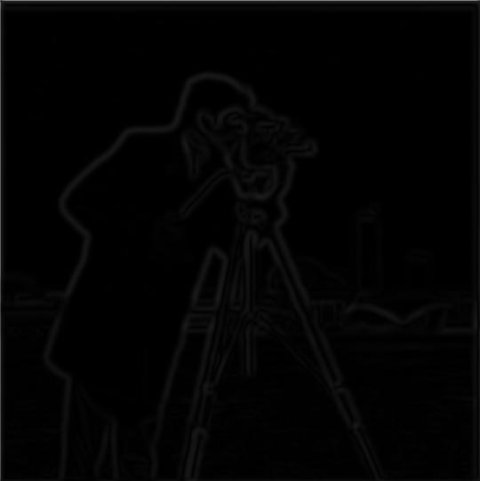
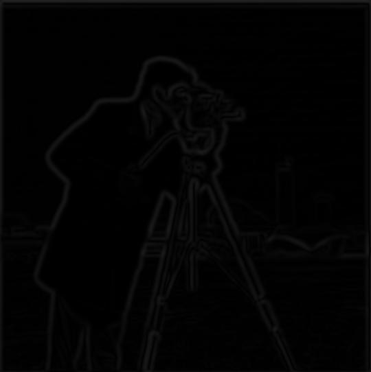
After getting the derivative results, we can further detect the edges. Before we do that we would need to first calculate the
magnitude of the image. This can be done through taking the square root of the squared sum of dx and dy.
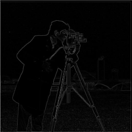
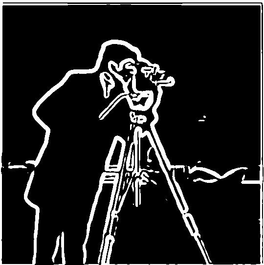
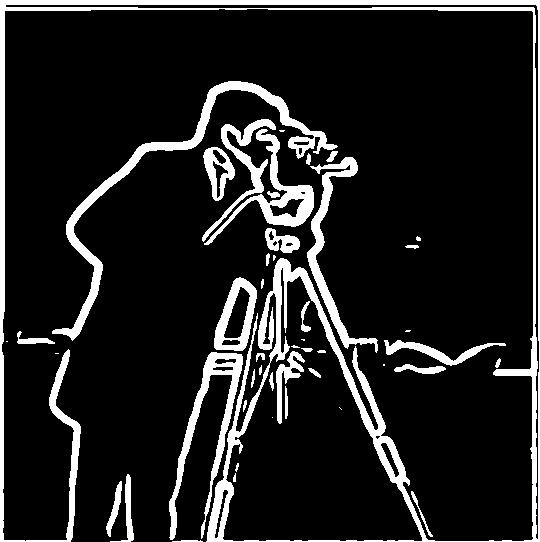
This is the gradient magnitude image that we get This is the edges that we detect, by binarizing the gradient magnitude image
Part 1.2: Derivative of Gaussian (DoG) Filter
We notice that the result from the previous part was pretty noisy. To improve on this, we can filter the image through a low pass filter, to reduce the higher frequencies.
There are two methods of conducting this. First being that we pass the gaussian filter through the image first, then taking the derivative.
The results are shown below.
Method 1: filtering the image first. Derivative of x resultMethod 1: filtering the image first. Derivative of y result
Method 1: filtering the image first. Magnitude imageMethod 1: filtering the image first. Edge image
The second method is first convolving the gaussian filter with the derivatives, then passing the new filters through the image. This method should yield the same result as the first.
Method 2: convolving derivative with filter first. Derivative of x resultMethod 2: convolving derivative with filter first. Derivative of y result
Method 2: convolving derivative with filter first. Magnitude imageMethod 2: convolving derivative with filter first. Edge image
Observations:
From these operations, we can see that the noise in the edge images have decreased greatly.
Part 2: Fun with Frequencies!
Part 2.1: Image "Sharpening"
In this portion, we are tasked to "sharpen" images. This process essentially extracts the high frequencies of an image and adds it back to the original image, with adjusted alpha.
In lecture, it was mentioned that there are two methods to complete this.
1. Adding the higher frequencies back with adjusted to alpha.
2. Calculate ((1 + alpha) * unit impluse - alpha * gaussian filter) then convolving that with the original image
In our case, we chose to go with the first method.
The original image of the Taj MahalSharpened image of the Taj Mahal
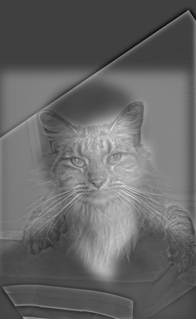
Original image of my catSharpened image of my cat.
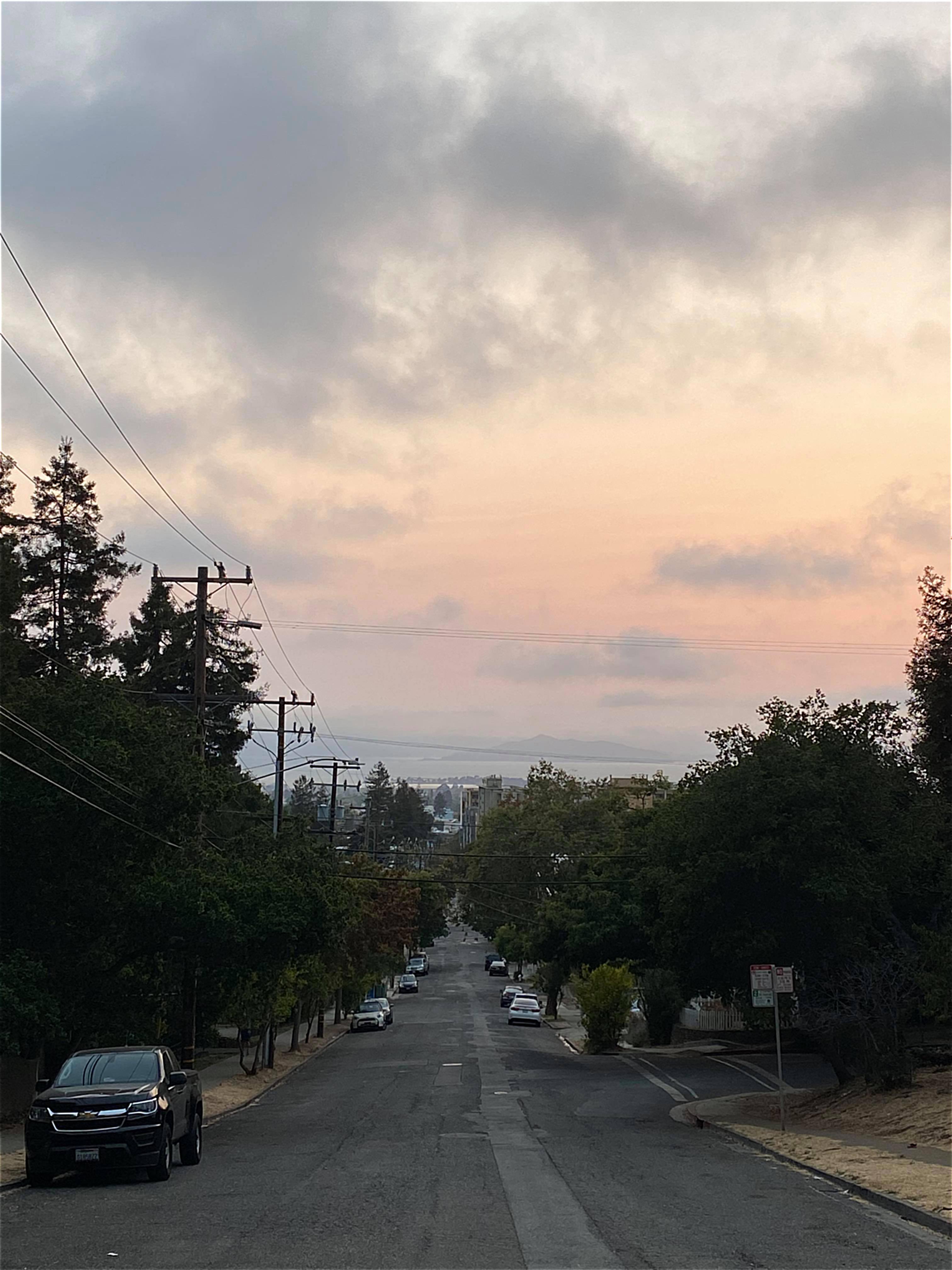
Original image of a sunset that I took. Sharpened image of that sunset.
Blur an image and sharpen
Picture of my cat sleeping.Blurred picture of my cat sleeping.Sharpened picture of that blurred one.
Observations:
Even though the sharpened image isn't identical to the original image. We can see an improvement to the clarity of the edges.
Part 2.2: Hybrid Images
With our knowledge in frequencies, we can also create hybrid images with them! This is by taking the high frequency of one image and overlaying that with the low frequency
of another image. The results are shown below.
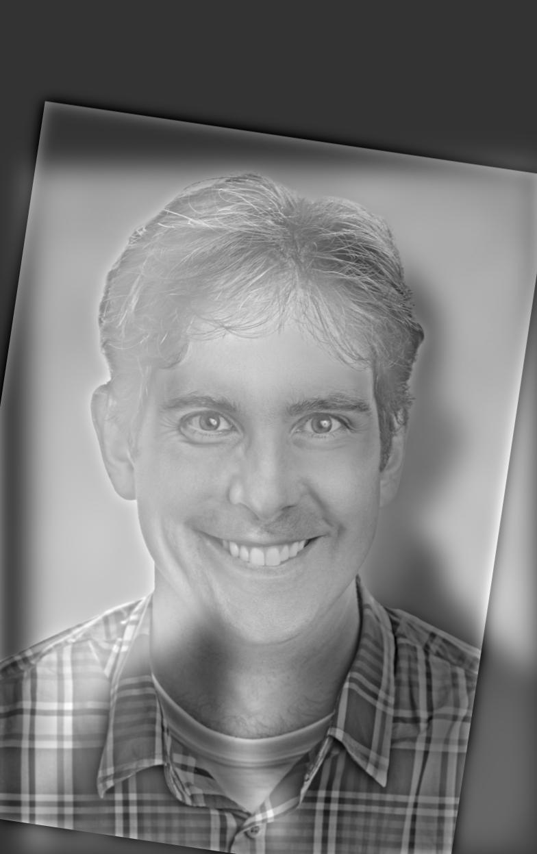
Picture of Derek.Picture of nutmeg.Dercat!
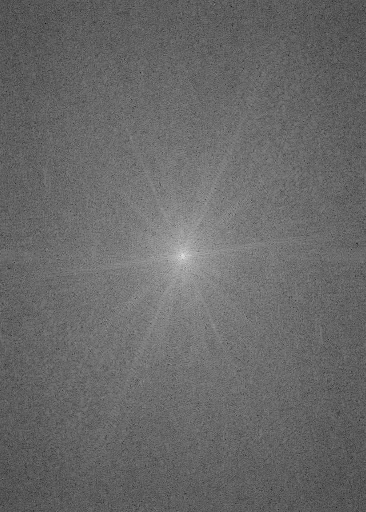
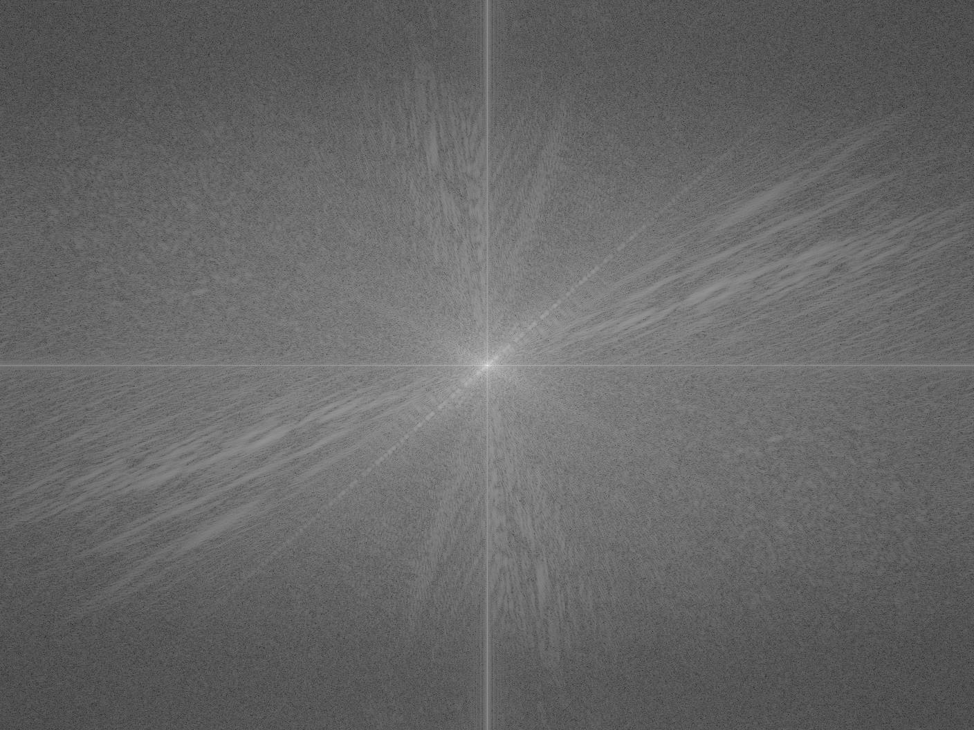
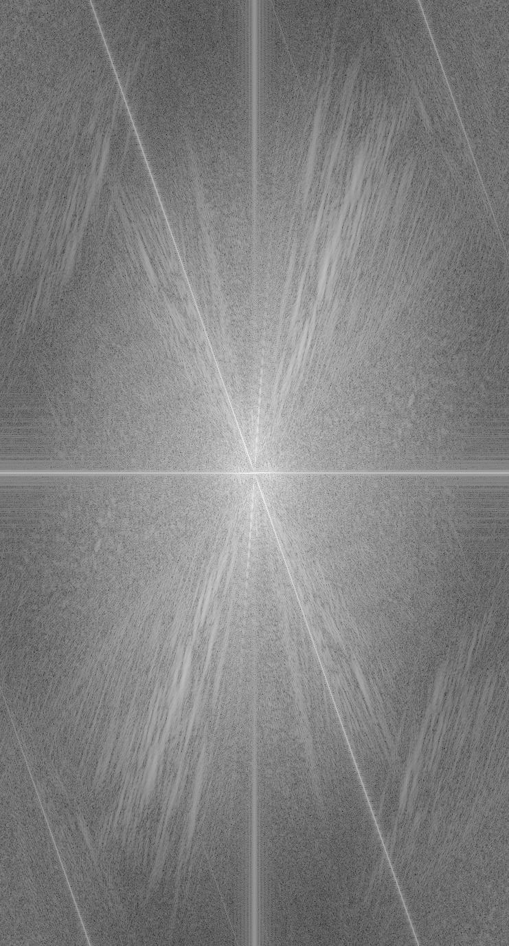
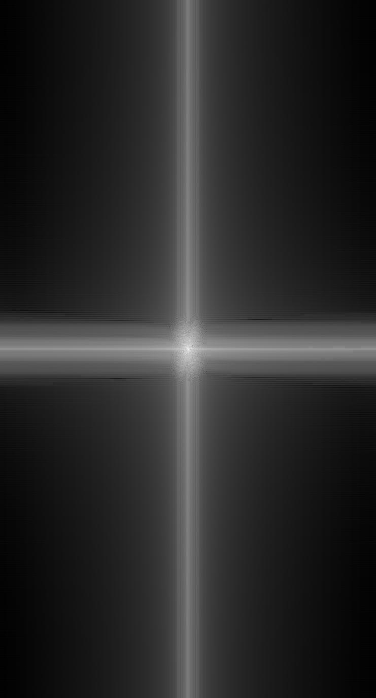
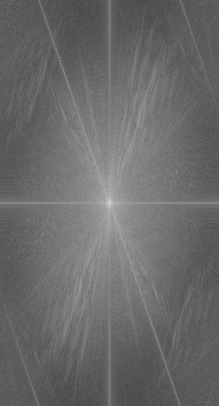
This is the log magnitude of the images at each step of the process.
Log magnitude of Derek's image.Log magnitude of nutmeg's image.
Log magnitude of Derek's image blurred.Log magnitude of nutmeg's image blurred.Log magnitude of hybrid of Derek and nutmeg blurred.
These are some fun creations that I made:
Professor Garnero
Picture of Professor Denero.Picture of Professor Garcia.Garnero!
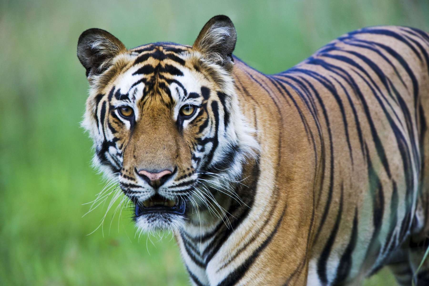
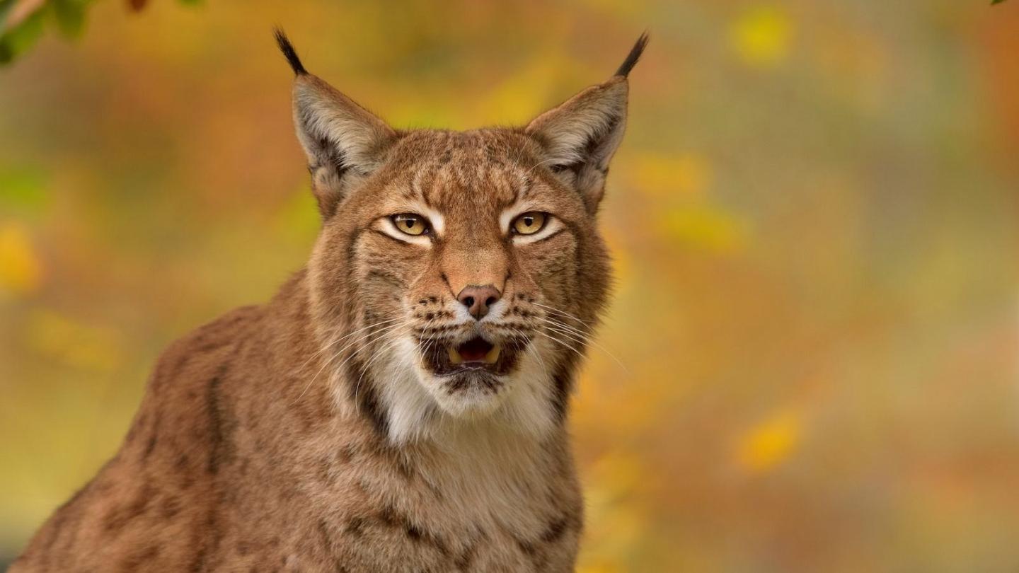
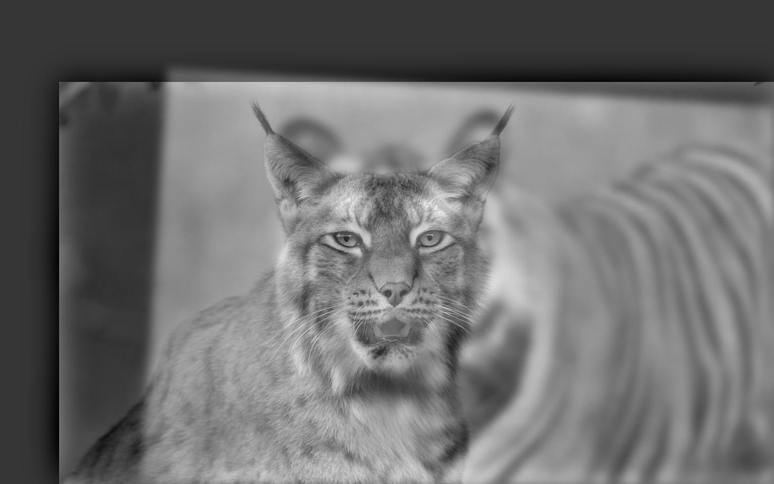
Lyger
Picture of a tiger.Picture of a lynx.Lyger!
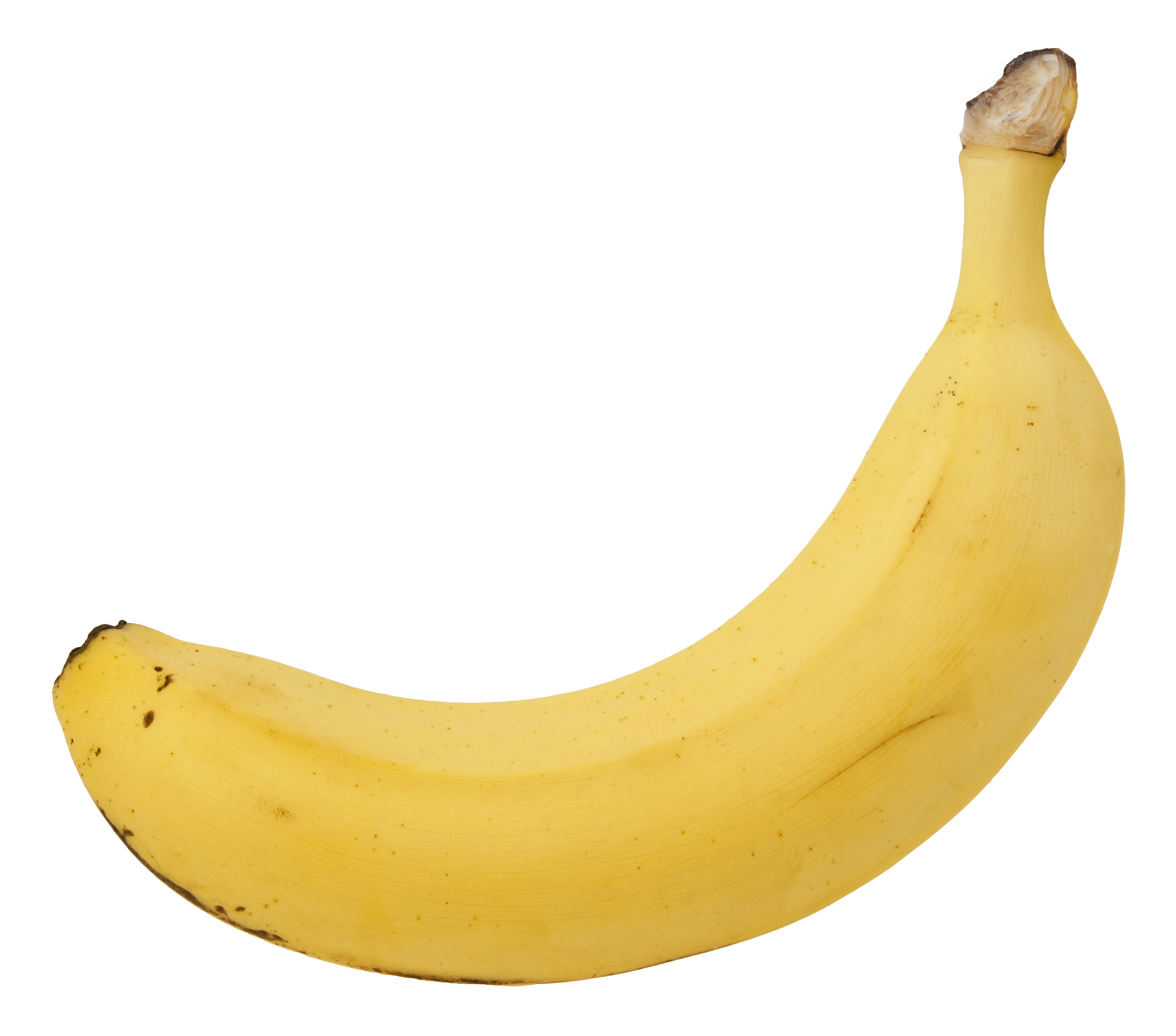
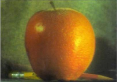
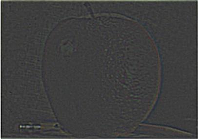
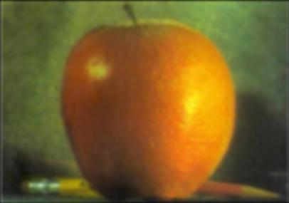
Here is a failed case of hybriding an image
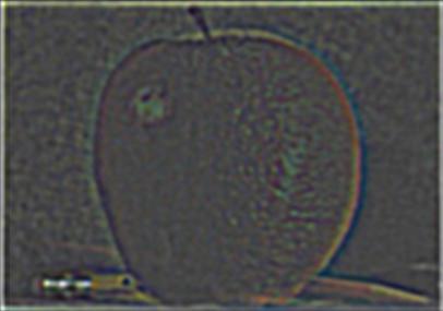
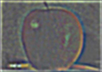
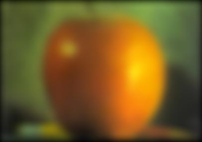
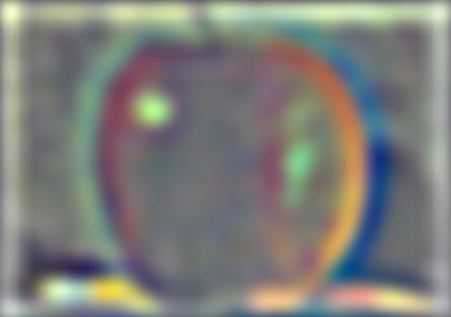
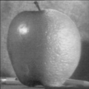
Picture of an apple.Picture of a banana.Banapple?
As we can see in the hybrid image, this is a failed case. This is due to the fact that we can't even notice the banana in the photo!
Multi-resolution Blending and the Oraple journey
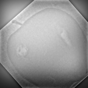
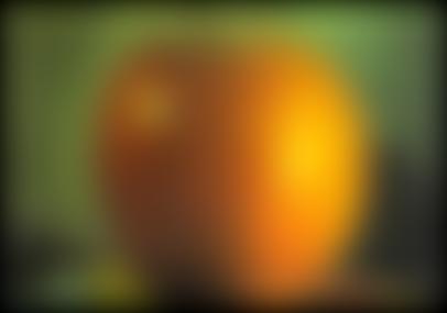
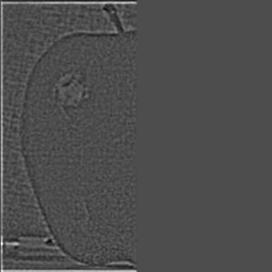
Part 2.3: Gaussian and Laplacian Stacks
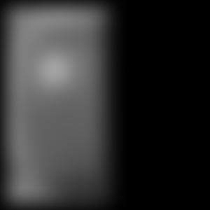
In this part we are constructing the Gaussian and the Laplacian stacks. The way to construct the Gaussian stack is that we increase the sigma at each level of the stack, thus
the sigma at each level of the stack will be 2 ** l. On the other hand, the method of constructing the Laplacian stack would be to simply subtract two consecutive levels of a
Gaussian stack. Thus, level l of a Laplacian stack will be level l + 1 - level l of the Gaussian stack.
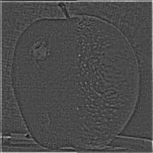
Level 0 of the Gaussian Stack.Level 0 of the Laplacian Stack.
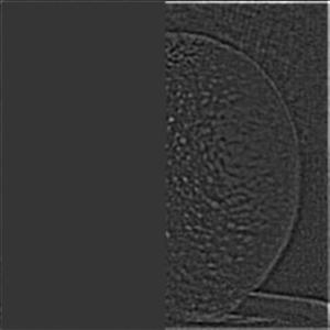
Level 1 of the Gaussian Stack.Level 1 of the Laplacian Stack.
Level 2 of the Gaussian Stack.Level 2 of the Laplacian Stack.
Level 3 of the Gaussian Stack.Level 3 of the Laplacian Stack.
Level 4 of the Gaussian Stack.Level 4 of the Laplacian Stack.
We can see that the Gaussian and the Laplacian yields the same result! To be noted the recreated of figure 3.4.2, is shown in the next portion.
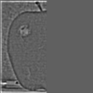
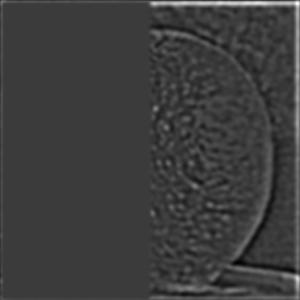
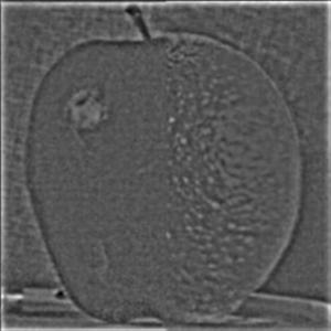
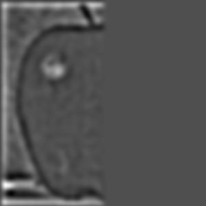
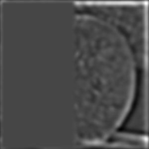
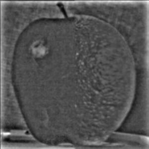
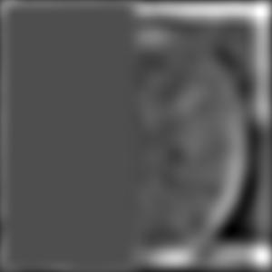
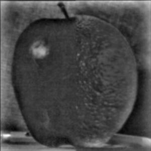
Part 2.4: Multiresolution Blending (a.k.a. the oraple!)
Level 0 of the Gaussian Stack.Level 0 of the Laplacian Stack. Level 0 of the combined stacks.
Level 1 of the Gaussian Stack.Level 1 of the Laplacian Stack. Level 1 of the combined stacks.
Level 2 of the Gaussian Stack.Level 2 of the Laplacian Stack. Level 2 of the combined stacks.
Level 3 of the Gaussian Stack.Level 3 of the Laplacian Stack. Level 3 of the combined stacks.
Level 4 of the Gaussian Stack.Level 4 of the Laplacian Stack. Level 4 of the combined stacks.
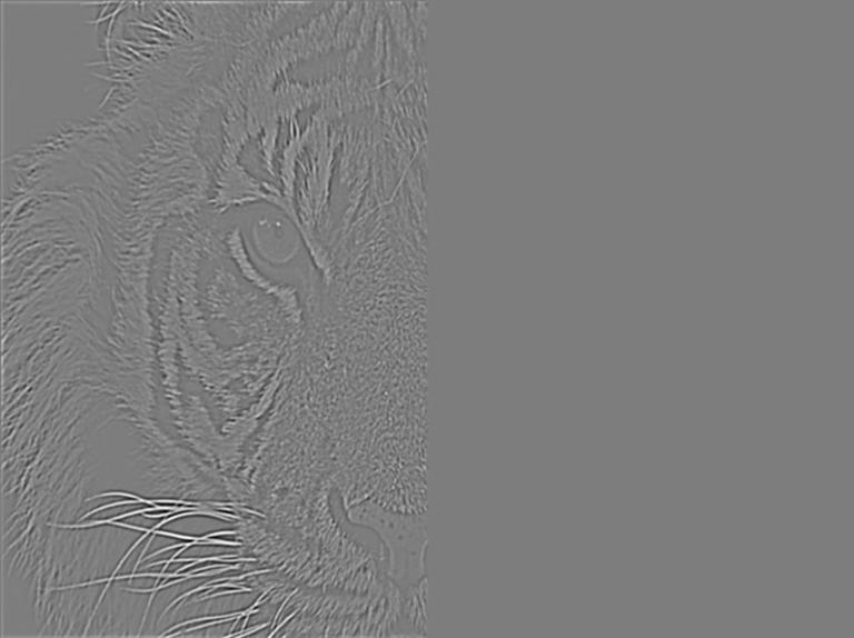
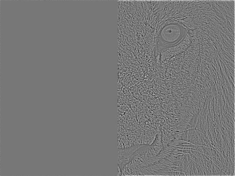
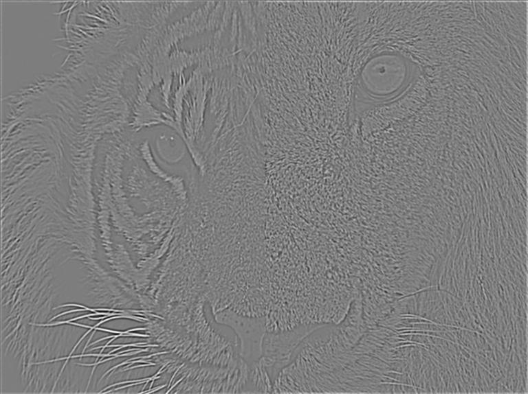
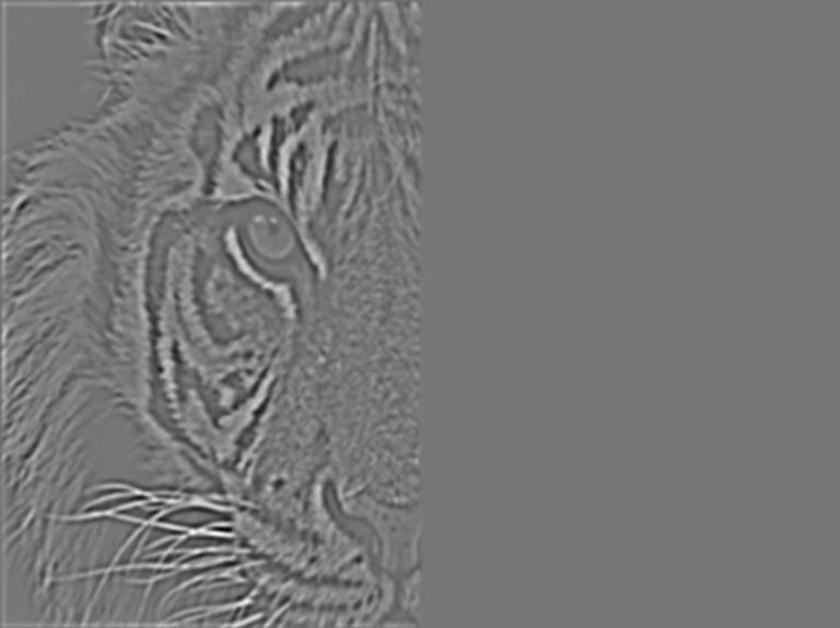
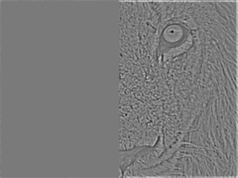
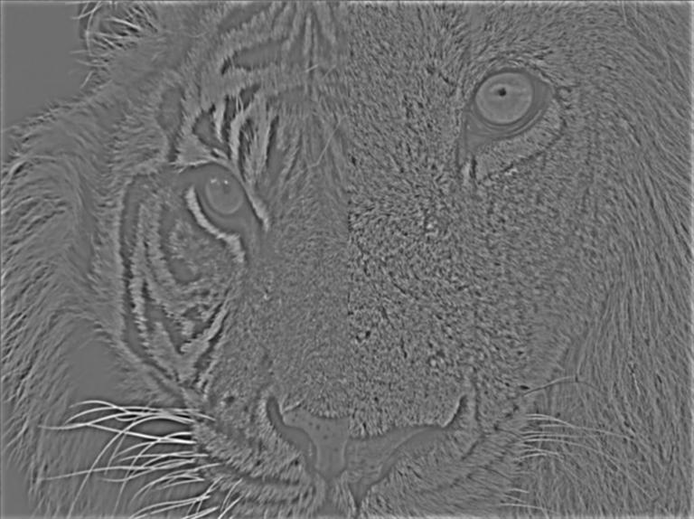
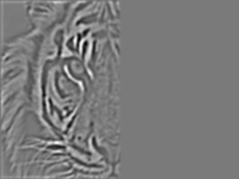
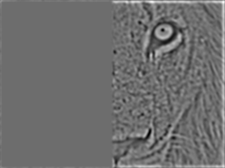
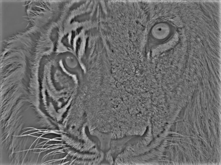
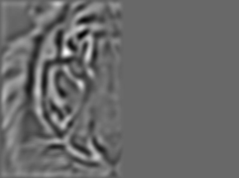
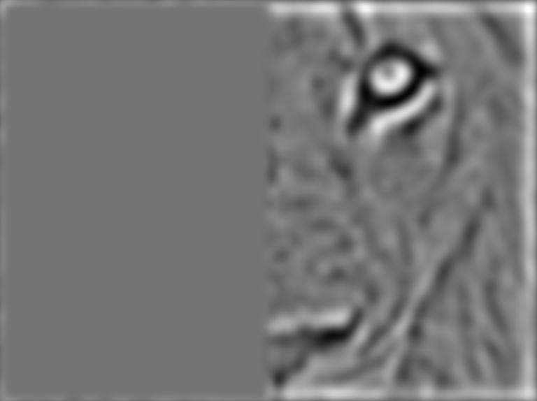
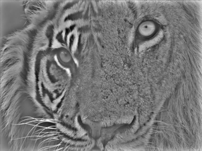
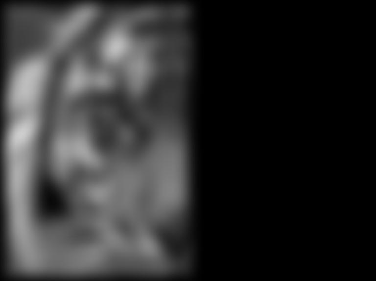
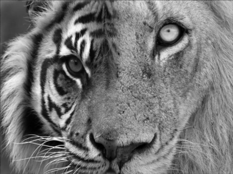
Tiger and Lion Combination
Level 0 of the Gaussian Stack.Level 0 of the Laplacian Stack. Level 0 of the combined stacks.
Level 1 of the Gaussian Stack.Level 1 of the Laplacian Stack. Level 1 of the combined stacks.
Level 2 of the Gaussian Stack.Level 2 of the Laplacian Stack. Level 2 of the combined stacks.
Level 3 of the Gaussian Stack.Level 3 of the Laplacian Stack. Level 3 of the combined stacks.
Level 4 of the Gaussian Stack.Level 4 of the Laplacian Stack. Level 4 of the combined stacks.
Professor Denero and Sahai
Original image of Professor DeneroOriginal image of Professor SahaiProfessor Denhai
Discoveries:
The coolest part of this project is understanding that even though some operations may seem very complicated. But they are actually
just simple math and matrix operations!