CS194-26 Project 2
Fun with Filters and Frequencies
Sean Kwan, Fall 2021
Part 1: Fun with Filters
Part 1.1: Finite Difference Operator
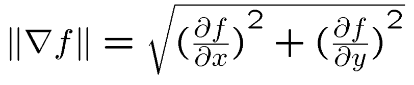
In order to compute the gradient magnitude of the image, we need:
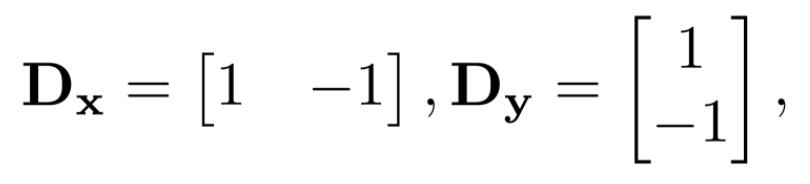
1. Partial Derivative with respect to X
2. Partial Derivative with respect to Y
However, since we are dealing with images in a discrete setting, we need an approximation for the partial derivatives. The approximation used for a partial derivative with respect to X in this project is simply the difference with respect to the next pixel, and similarly with Y.
Thus, to concisely and efficiently compute the partial derivatives of the image, we convolve the image with the respective partial derivative filter and mode='same' to preserve the original shape of the image. Since, we now have both the partial derivative with respect to X and Y, we can compute the gradient magnitude of the image by simply taking the square root of the sum of squares of the partial derivatives.
To get an even better understanding of partial derivatives and the gradient magnitude, shown below are examples of the effects of these functions on the image cameraman.png.
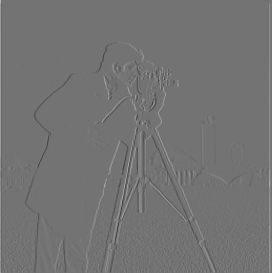
Partial Derivative with respect to X
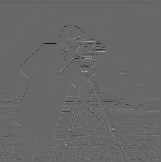
Partial Derivative with respect to Y
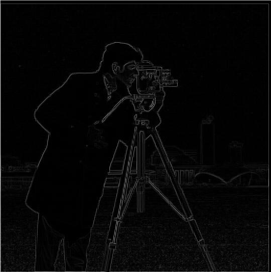
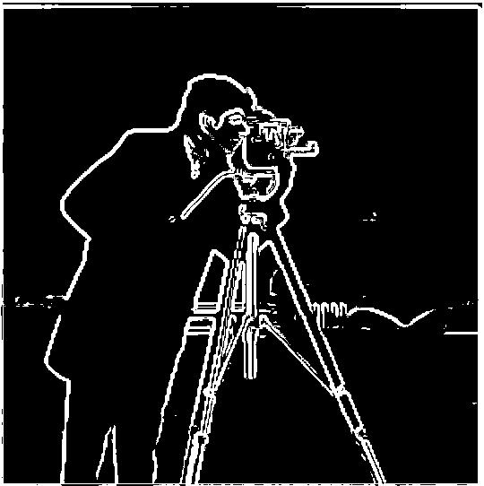
Gradient Magnitude
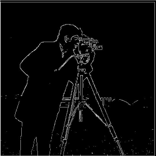
Binarized Gradient magnitude with threshold=0.1
Part 1.2: Derivative of Gaussian (DoG) Filter
The issue with the original image is that there is a lot of noise which results in the binarized gradient magnitude image still leaving in the residual noise. To tackle this issue, I introduced a low-pass filter using a Gaussian filter to pre-process the noisy image and get rid of the noise.
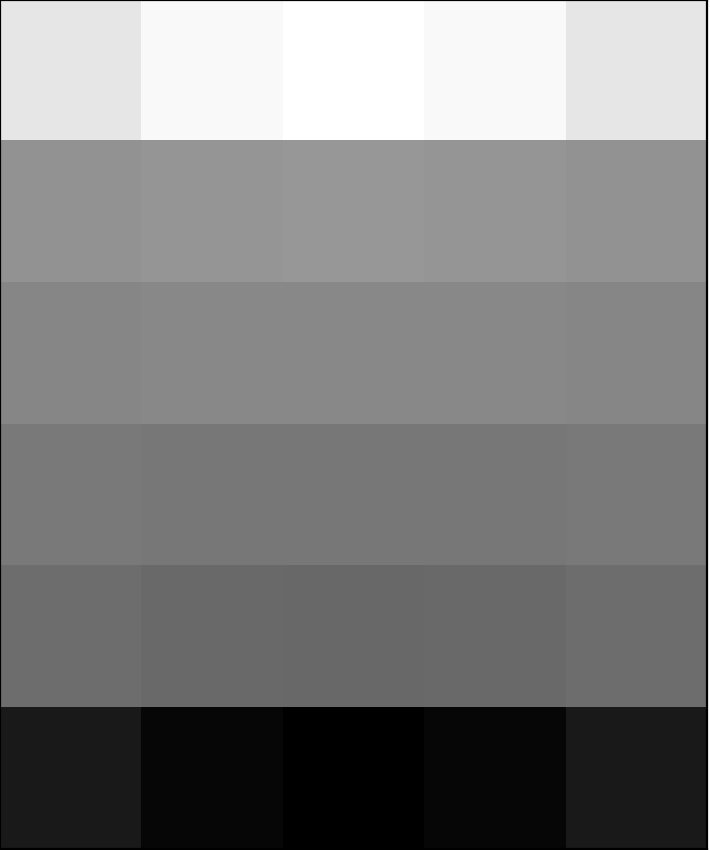
Gaussian Pre-processed Result
The difference in results between this and the original is that the edges are much better defined due to the noise in the grass being removed beforehand. However, it's important to note that this requires two convolutions on the image We can reduce this to one convolution by creating a Derivative of Gaussians (DoG) and using the DoG filters on the image directly. This results in a binarized gradient magnitude image that is the same as the gaussian pre-processed image.

DoG X
DoG Y
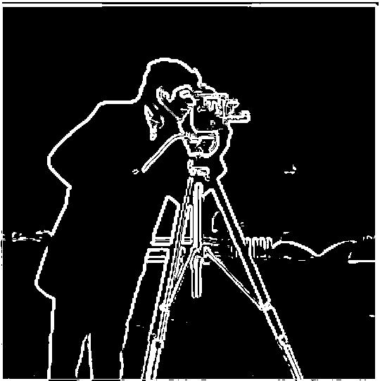
DoG Filter Result
Part 2: Fun with Frequencies
Part 2.1: Image "Sharpening"
The Gaussian low-pass filter that we developed in Part 1 helped create a blurry image which kept only the lower frequency parts (removed the high frequency parts) of the image. We can subtract the blurry image from the original to create an image which only retains the high frequency parts of the image. This high frequency image can be added to the original image with some weight, alpha, to create a "sharpened" image. This can then be condensed into one convolution called the Unsharp Mask Filter. The following images show the results of the Unsharp Mask Filter.
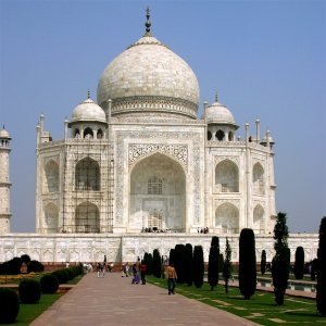
Original Taj
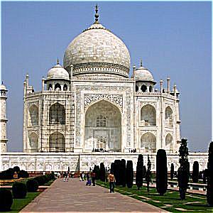
Sharp Taj
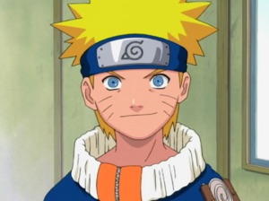
Original Naruto
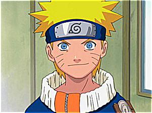
Sharp Naruto
The effects of the Unsharp Mask Filter on blurry images definitely seems to have a "sharpening" effect as shown from the photos above. However, when we have an image that is already sharp, blur it, then apply the Unsharp Mask Filter we see that the final image is not as clear as the original sharp image. This is because high frequency values are lost from the blurring process which can not be recovered with the Unsharp Mask Filter.
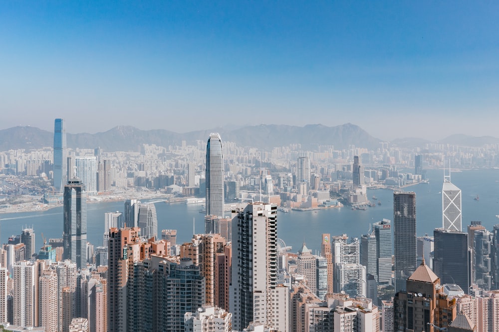
Sharp Hong Kong Skyline

Blurred Hong Kong Skyline
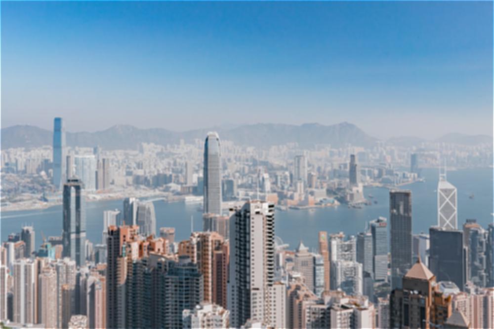
Sharpened Blurred Hong Kong Skyline
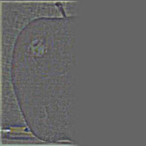
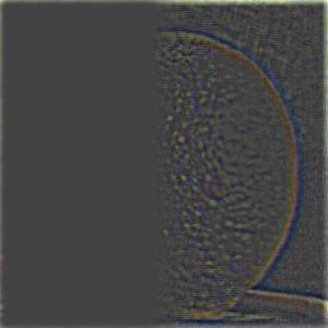
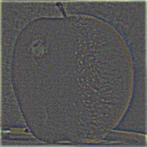
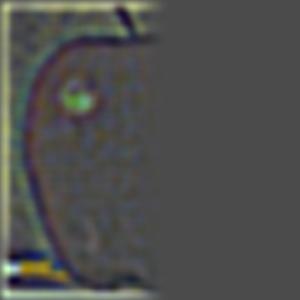
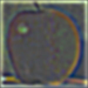
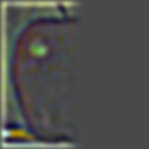
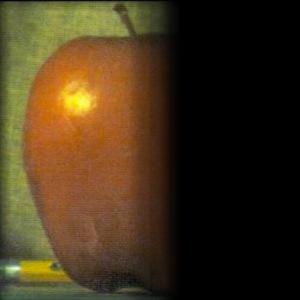
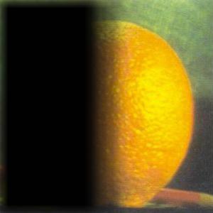
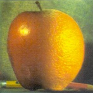
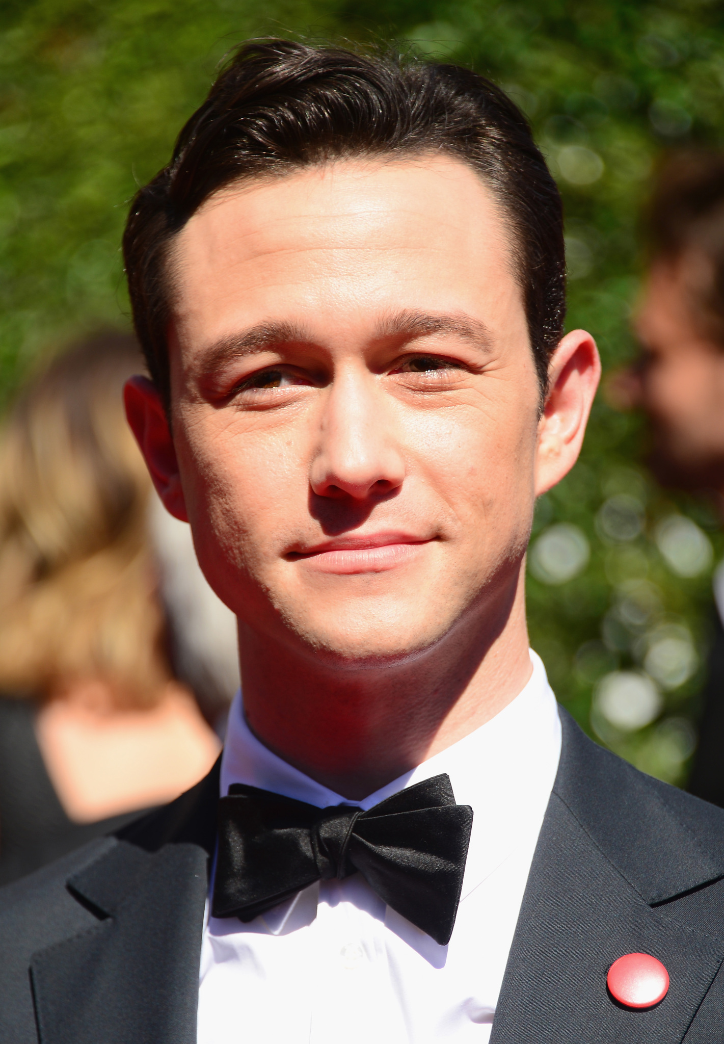
Part 2.2: Hybrid Images
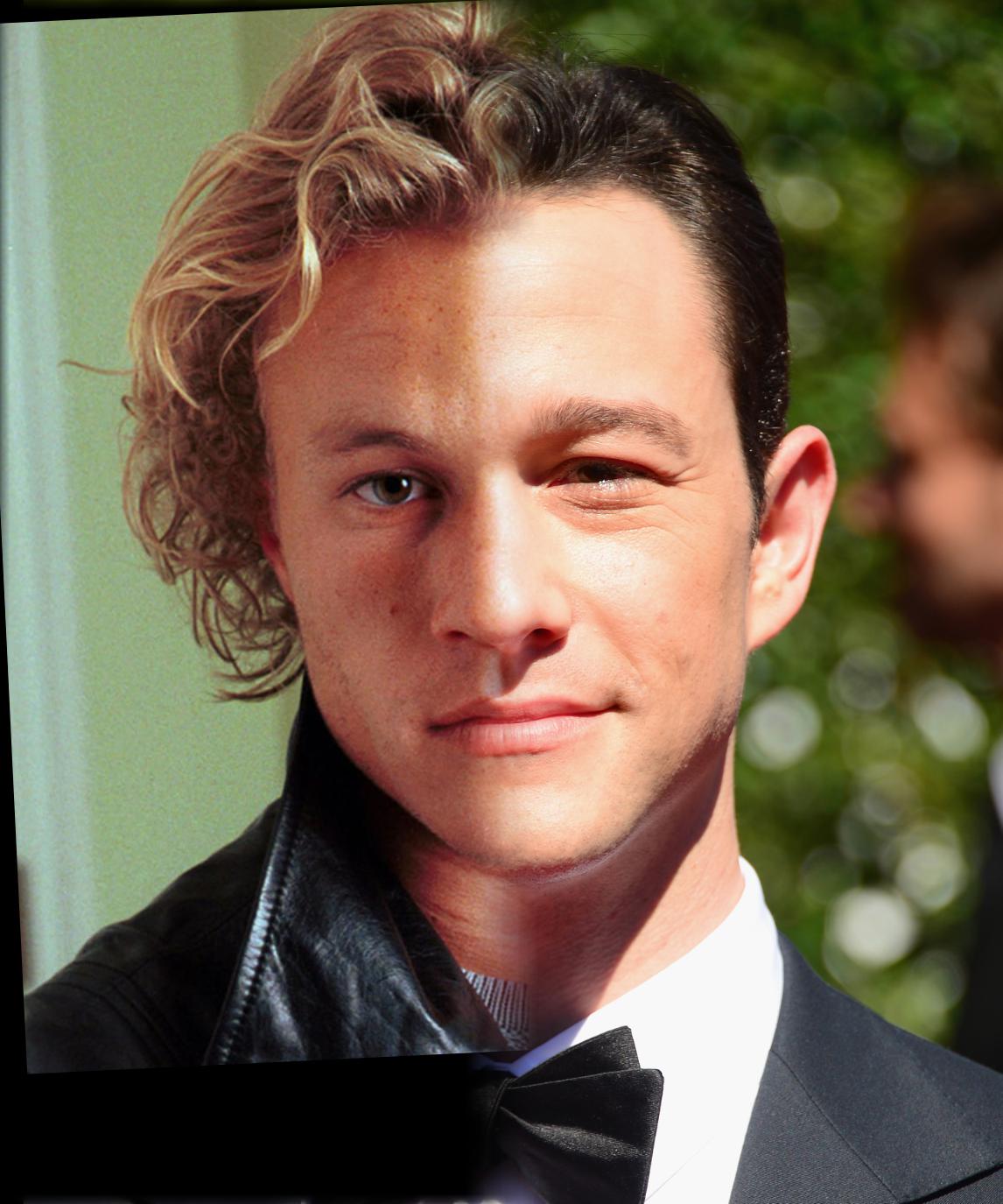
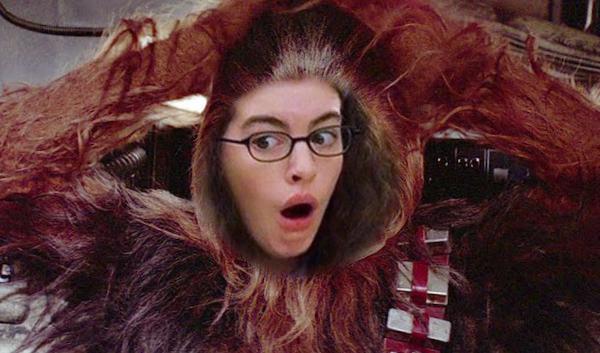
For Hybrid Images, we combine the knowledge that we learned from the previous parts by using both the low-pass and the high-pass filter. The low-pass image will be the image that we will be able to see from afar, whereas the high-pass image will be the image we can see from up close. This combination of a low-pass image with a high-pass image creates the hybrid images as shown below.
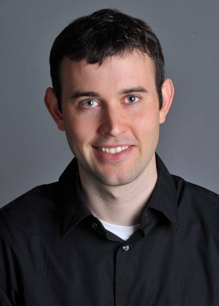
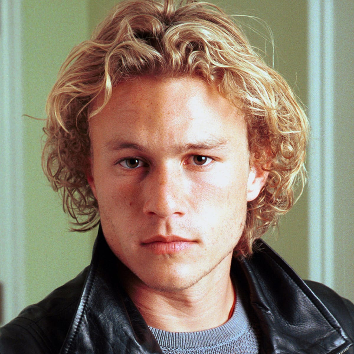
Derek
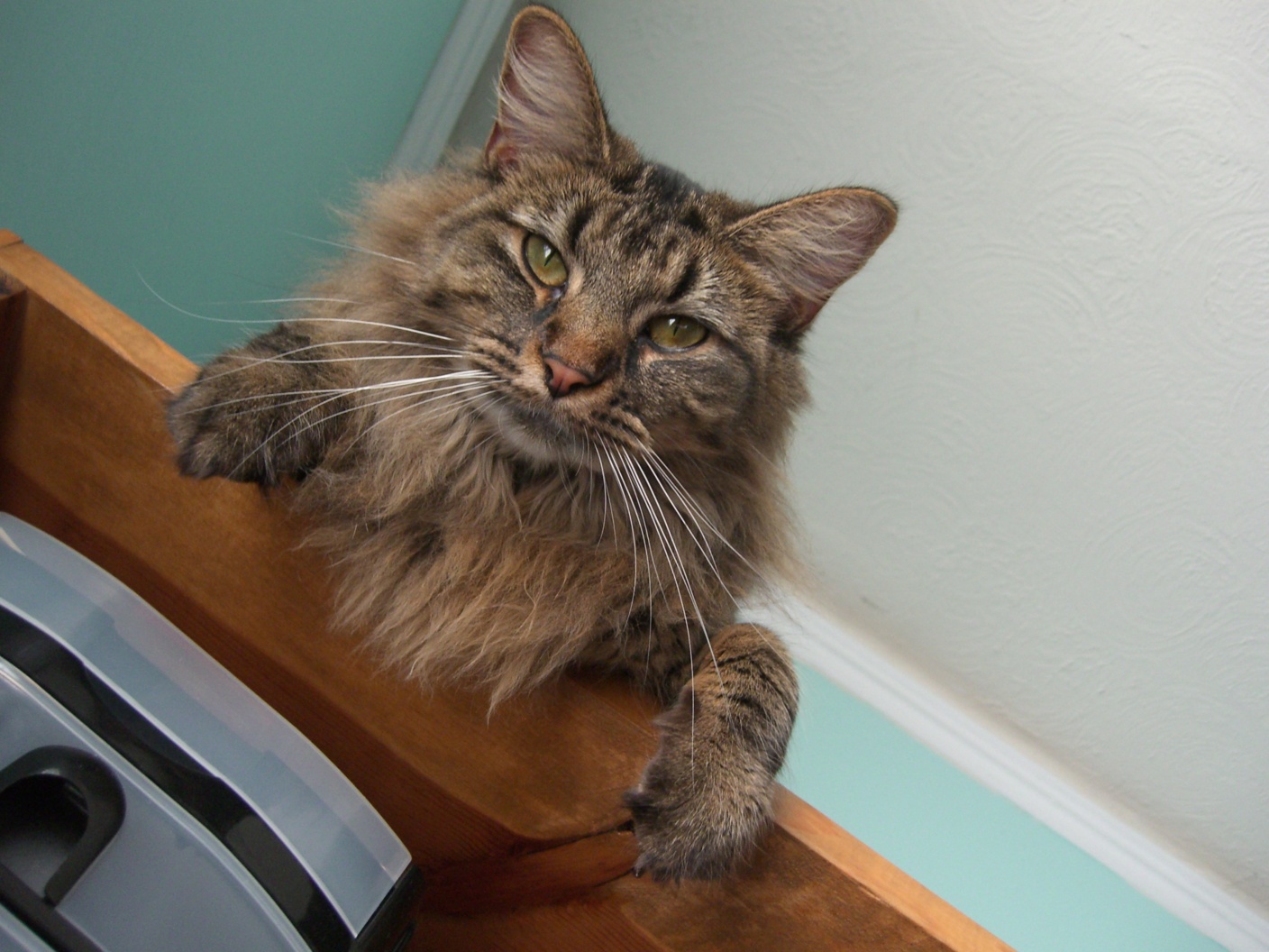
Nutmeg
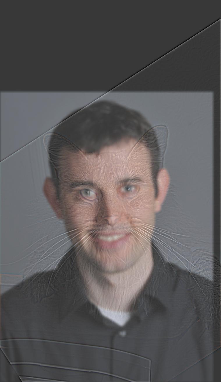
Hybrid Nutmeg Derek
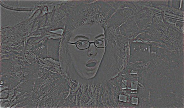
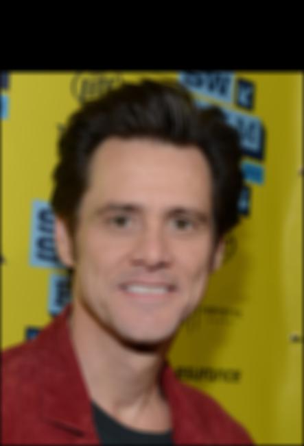
This is an example of the low-pass Jim Carrey photo with a high-pass The Mask photo to create an image which shows both sides of Jim Carrey's character in his iconic movie The Mask. This filtering was done with colored images through separating the image into its corresponding R, G, B channels and doing the filtering on each channel separately, then recombining the three filtered channels back into one filtered image.
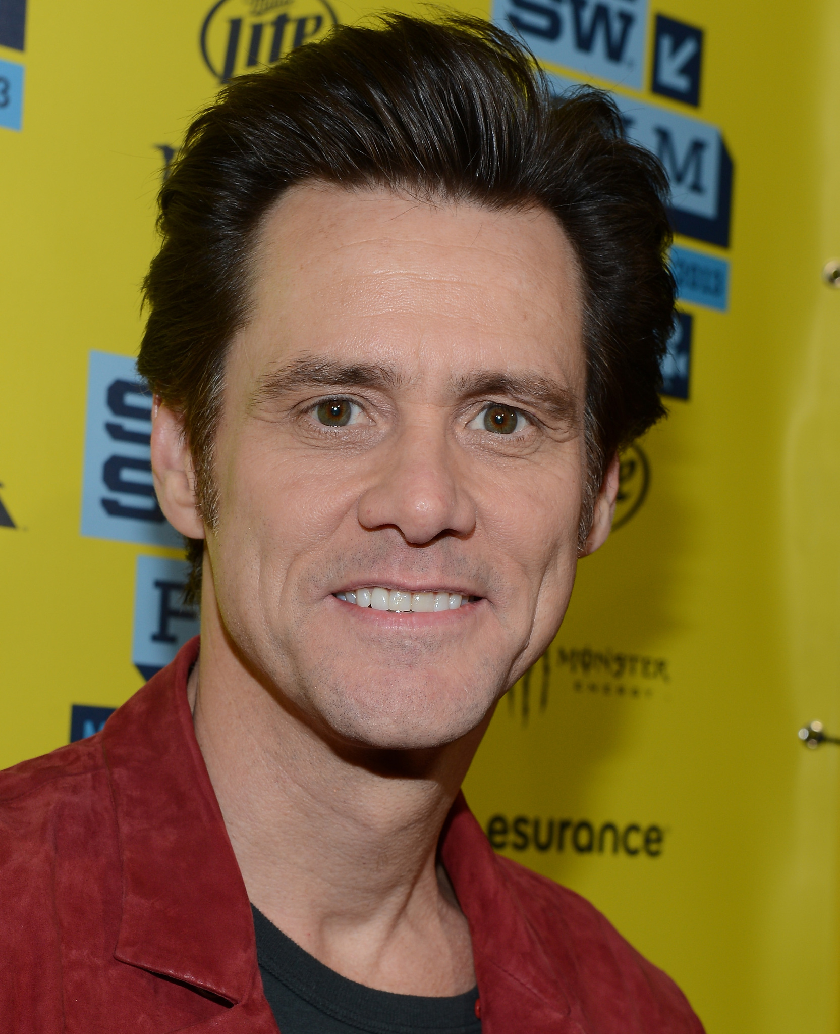
Jim Carrey
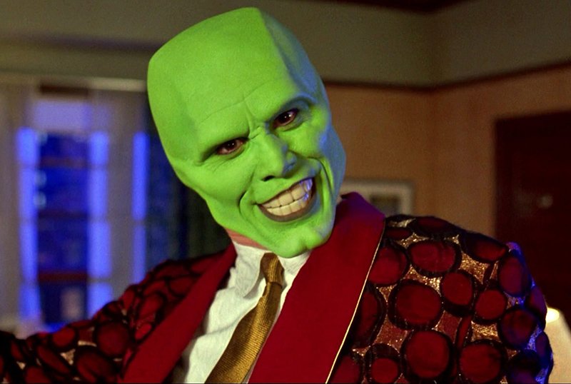
The Mask
Hybrid Jim Carrey The Mask
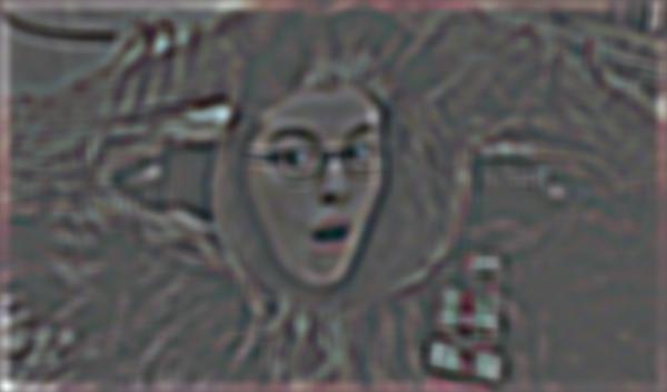
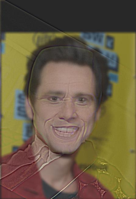
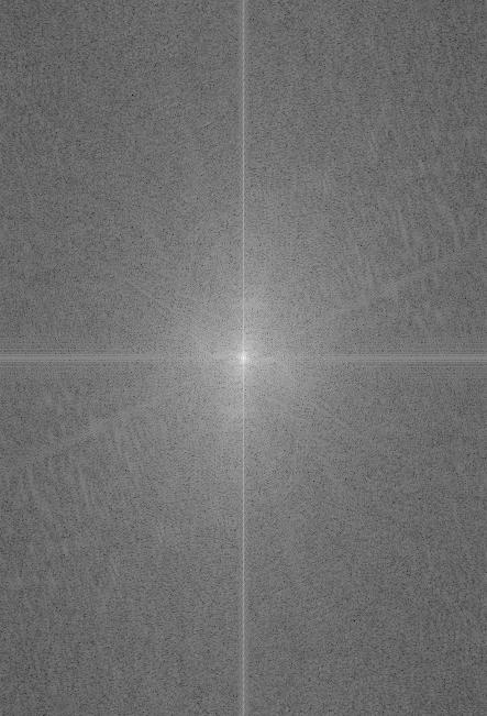
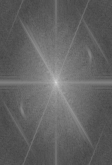
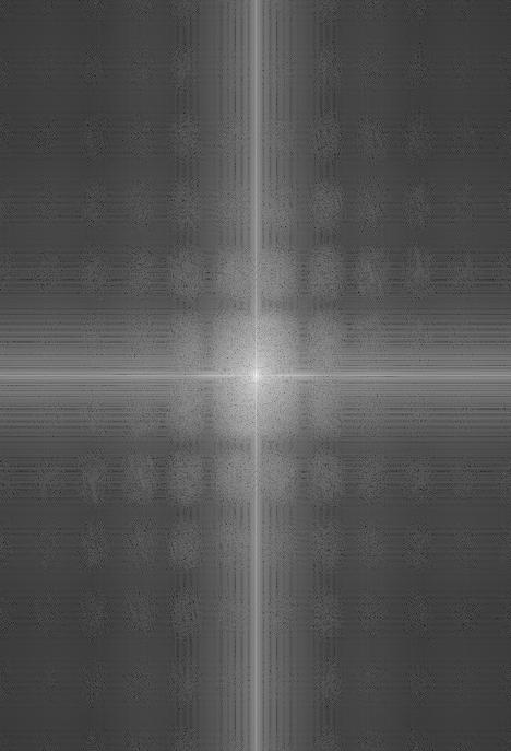
This is my favorite example, below is the entire process with the corresponding Fourier transform images for the original images, the filtered images and the final hybrid image.
Jim Carrey
Fourier Carrey
The Mask
Fourier The Mask
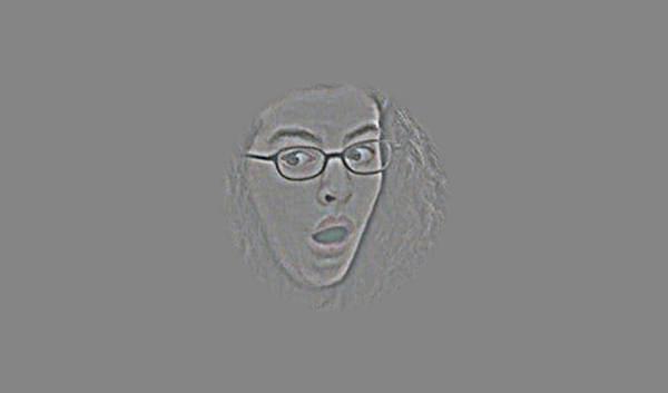
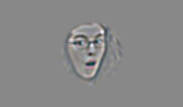
Low-pass Carrey
Fourier Low-pass Carrey
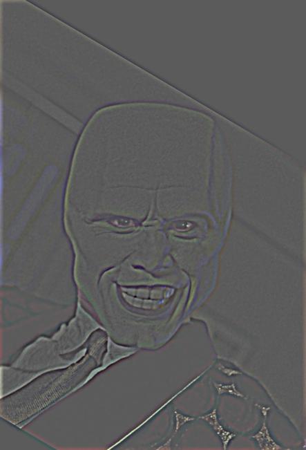
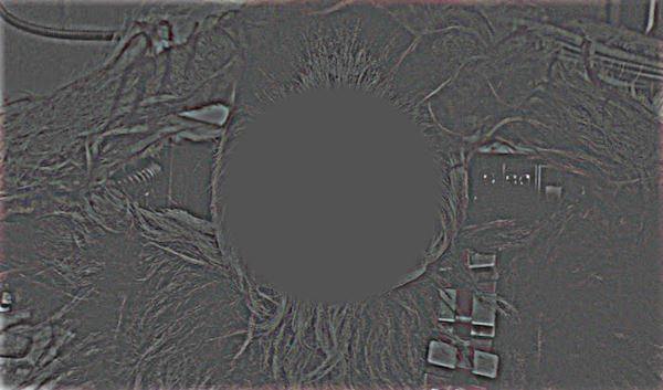
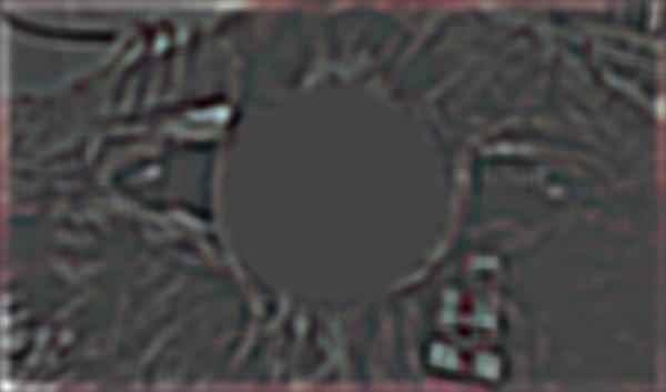
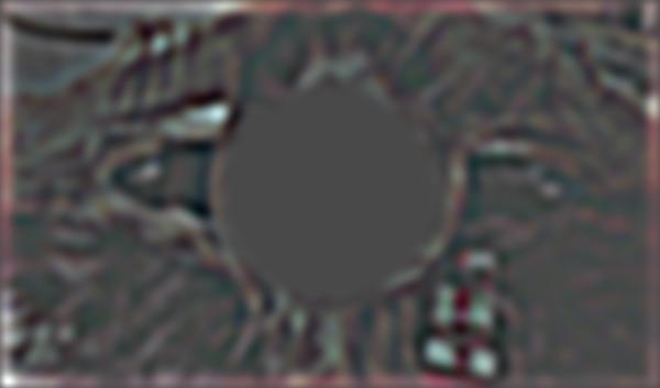
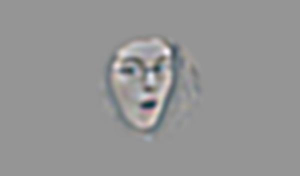
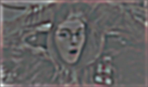
High-pass The Mask
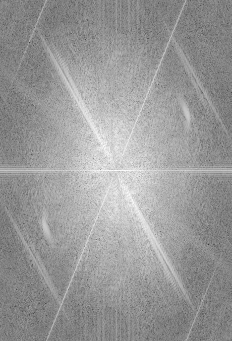
Fourier High-pass The Mask
Hybrid Carrey The Mask
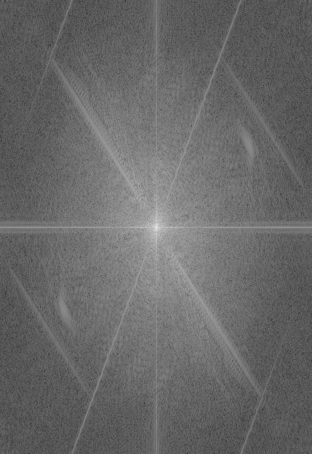
Fourier Hybrid Carrey The Mask
However, hybrid images do not always work as evidence by this failure example of me trying to combine Bruce Lee and Tron Legacy. I suspect that the slightly different poses caused the image to not match up well, in addition, there is quite a big difference in terms of the brightness of the photos which could also contribute to this failed hybrid image.
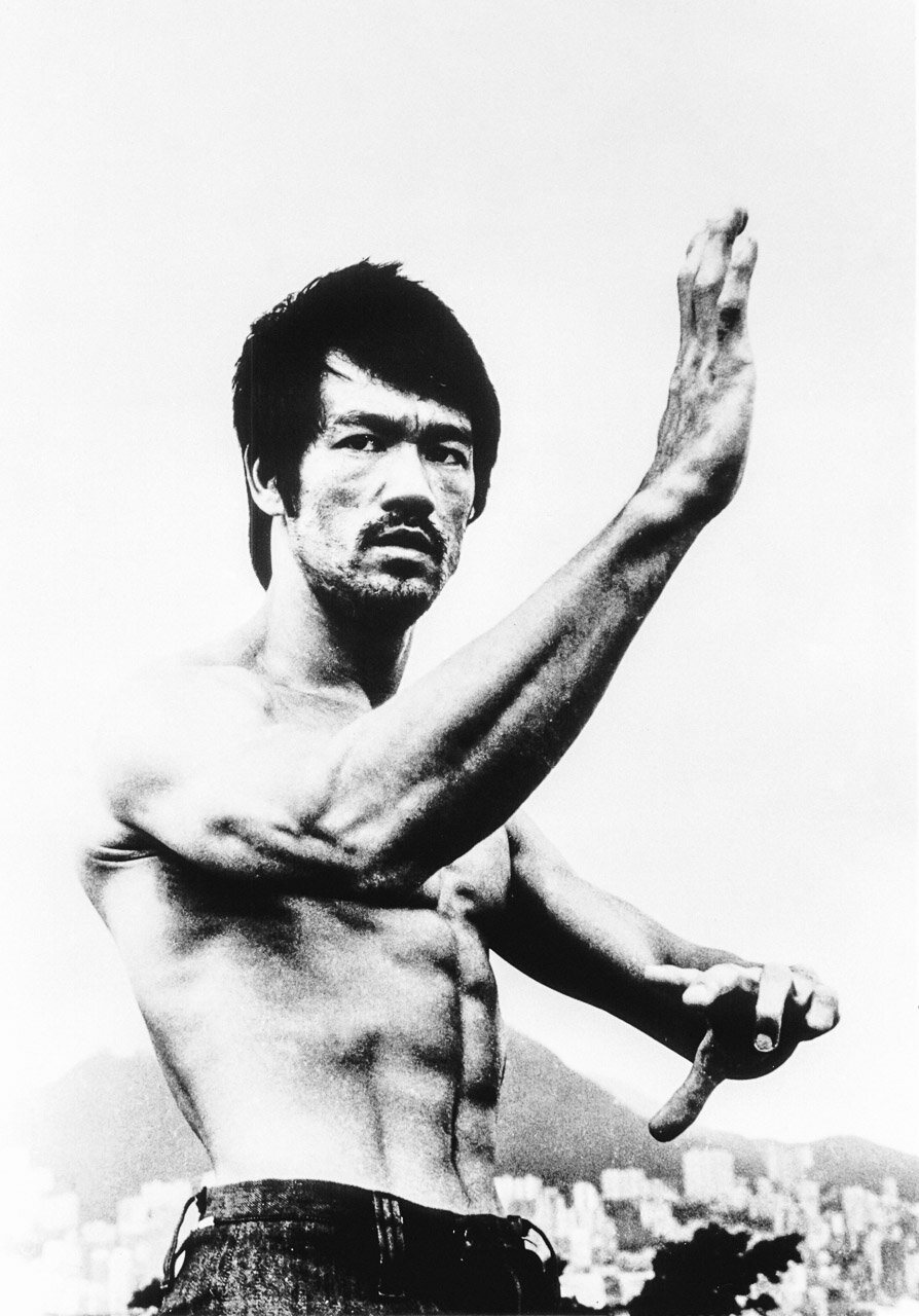
Bruce Lee
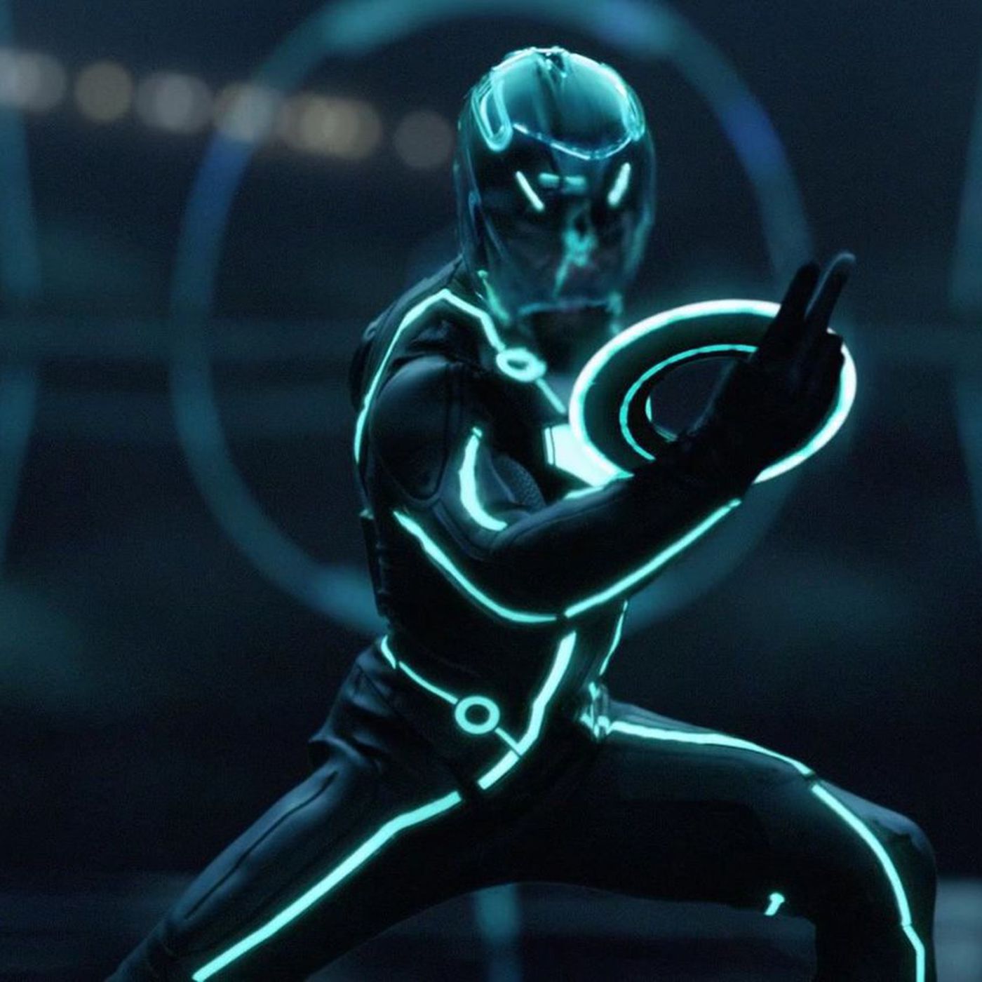
Tron
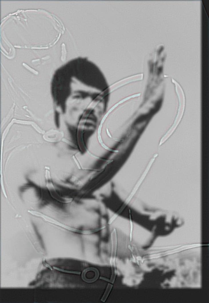
Failed Hybrid Bruce Lee Tron