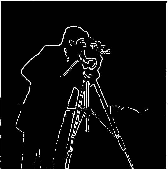
In this part of the project, we developed a finite difference filter and a derivative of gaussians filter that gave us the gradient magnitude image.
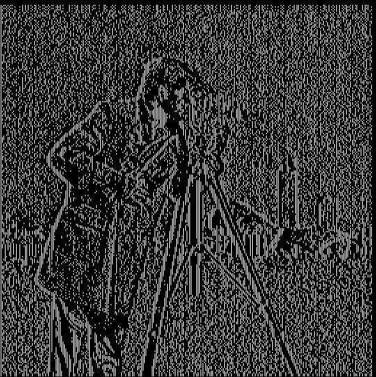
In this part, we convolved the image Cameraman with the finite difference operators on the x-axis and y-axis to find the gradient magnitude image. Note that the finite difference operators are the following: D_x = [ 1, -1] and D_y = [[1],[-1]]
In order to find the gradient on an image, we treat each image as a 3-dimensional object, where each pixel value acts as the height. Since photos are discrete, we have to find the derivative in a discrete manner: the best way to do this is by relying on the fact that $$\frac{df(x)}{dx} = \frac{f(x)-f(x+\Delta)}{\Delta}.$$ Since we are working in a discrete field, we find the gradient by setting $\Delta$ to be 1. Note that to find the gradient, we have to find the partial derivatives in this manner with respect to x and with respect to y. Once we find the gradient, we are able to find the magnitude by taking the length of the gradient. Interestingly, we perform gradient magnitude computation on grayscale images, since color images usually have similar information across different color channels—furthermore, we don't want to be relying on different colors for our algorithm to work.
Here is the image convolved with D_y:
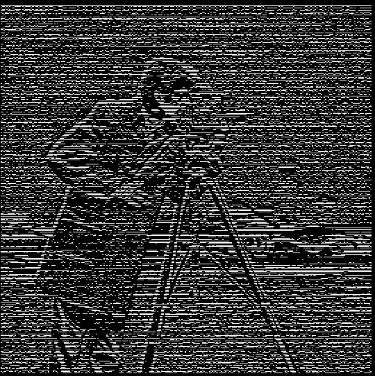
Here is the image convolved with D_x:
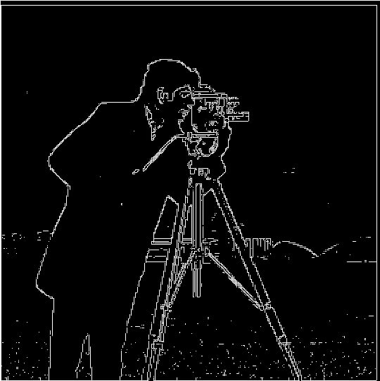
Here is the gradient magnitude image:

Here is the binarized gradient magnitude image, using a threshold of 0.1:
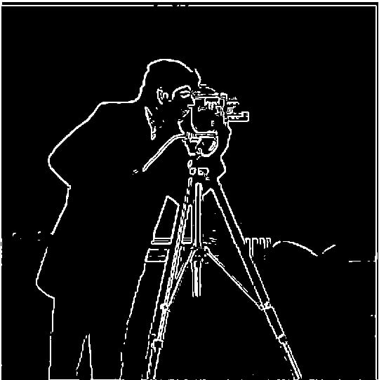
In this part, we first blurred the original image with a Gaussian filter of size 6 and sigma 1. Then, we convolved the blurred image with a finite difference operator.
Blurring the original image made the gradient magnitude image much clearer. Notice that the binaraized graident magnitude image in Part 1.1 still had small bits of background noise, even though the threshold was low enough to miss small sections of the cameraman. In the following image, the outline of the cameraman is still very clear while leaving out most of the background noise we noticed in the binarized gradient image in Part 1.1.
Another point of interest is the appearanceof the edges in Part 1.1 in comparison to the edges in this section. We can see that the edges of the gradient magnitude image in Part 1.1 are a bit choppy, with small sections of the cameraman's figure missing.
On the other hand, the edges of the blurred gradient magnitude image from this section are much more clear and well defined. Below we show the gradient magnitude image calculated using the derivative of Gaussian filter.
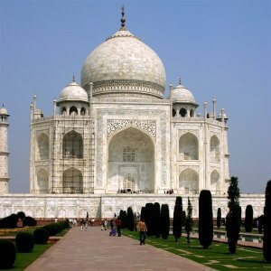
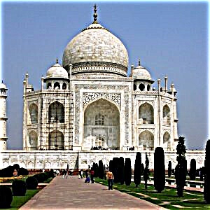
In this section, we attempted to "sharpen" a image by strengthening the high frequences inside the image. For instance, here is the original Taj:
Here is the Taj sharpened by finding the high frequencies with subtraction:

Here is the Taj sharpened by using the unsharp mask filter:
E
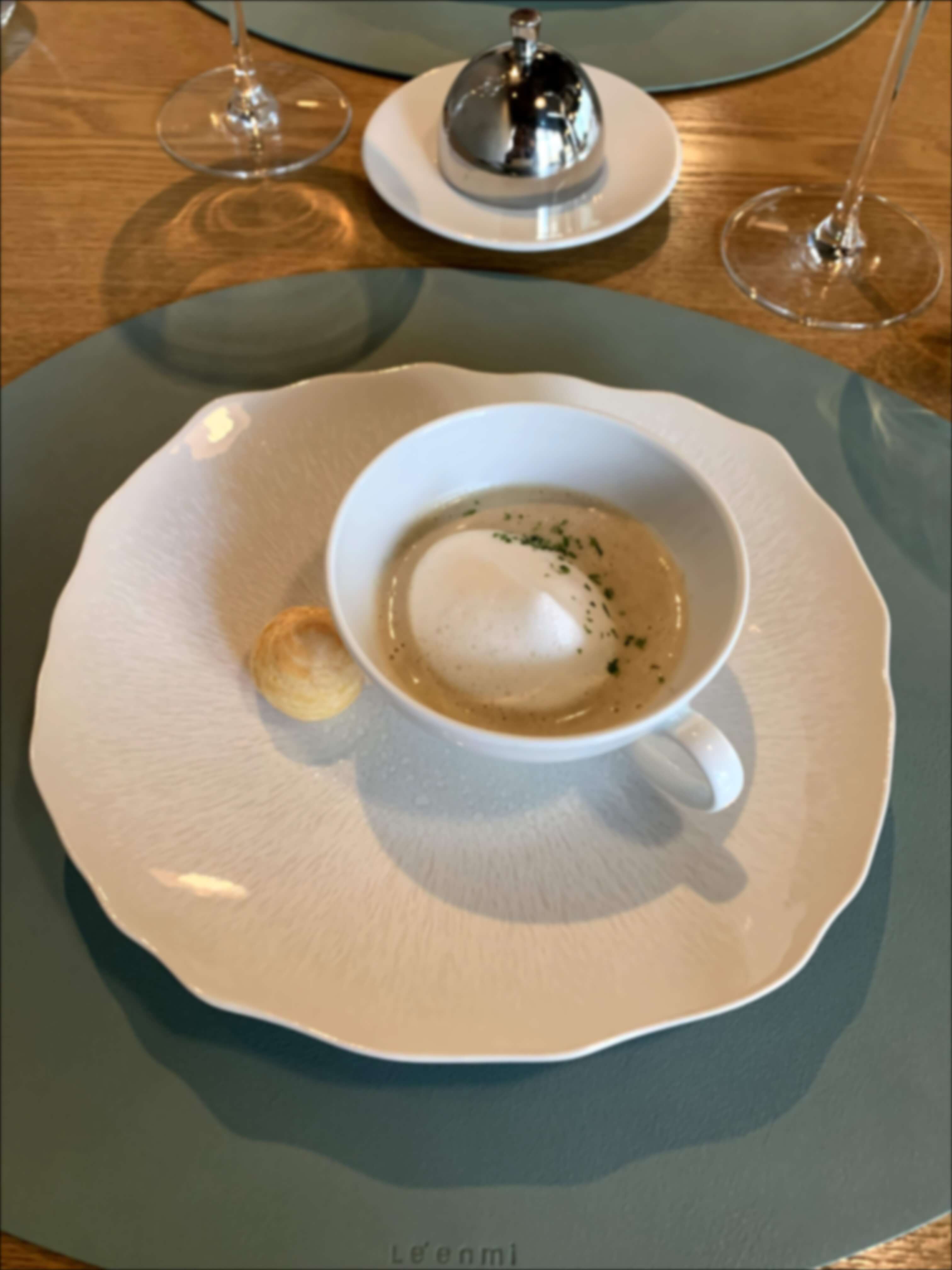
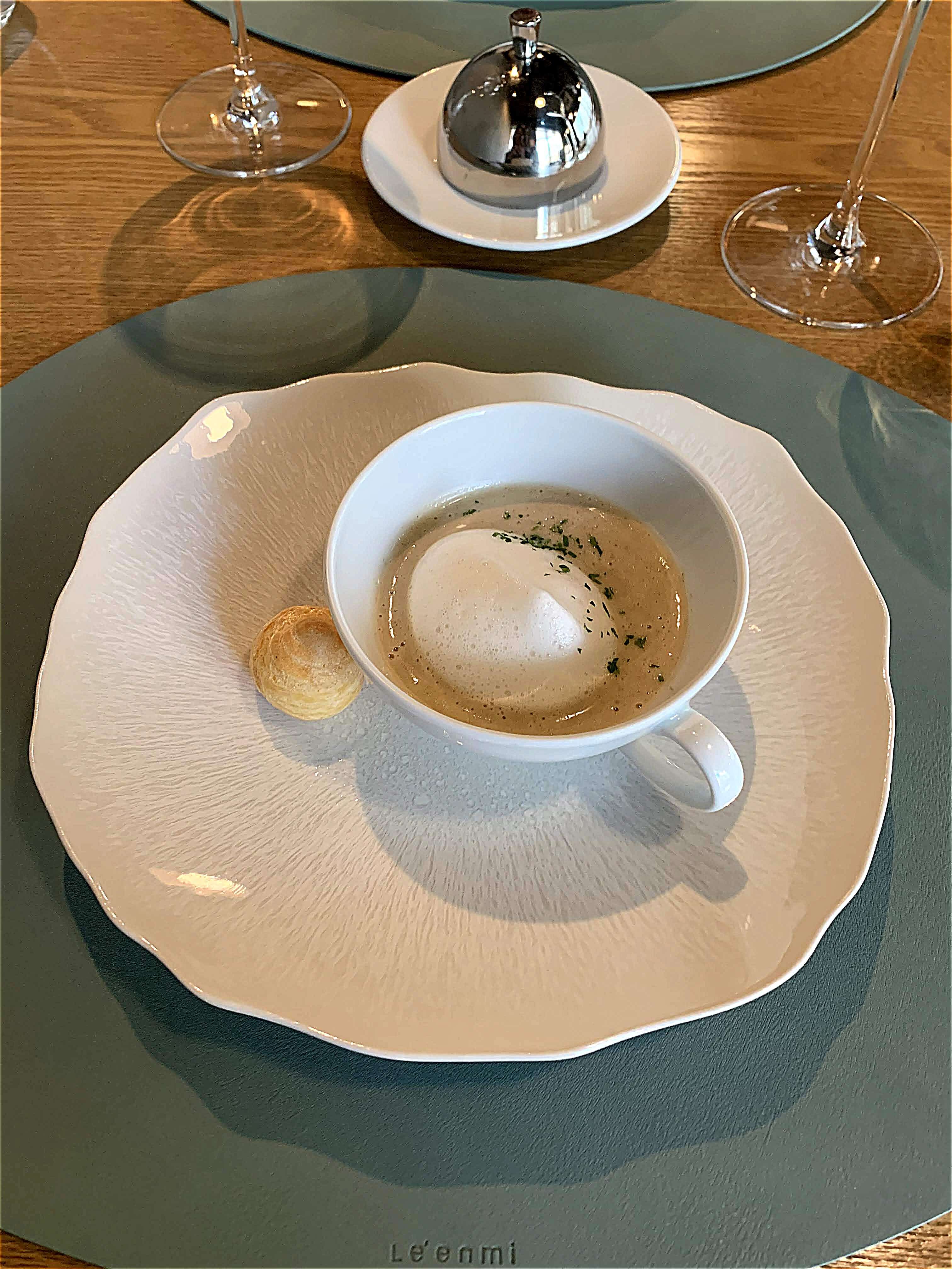
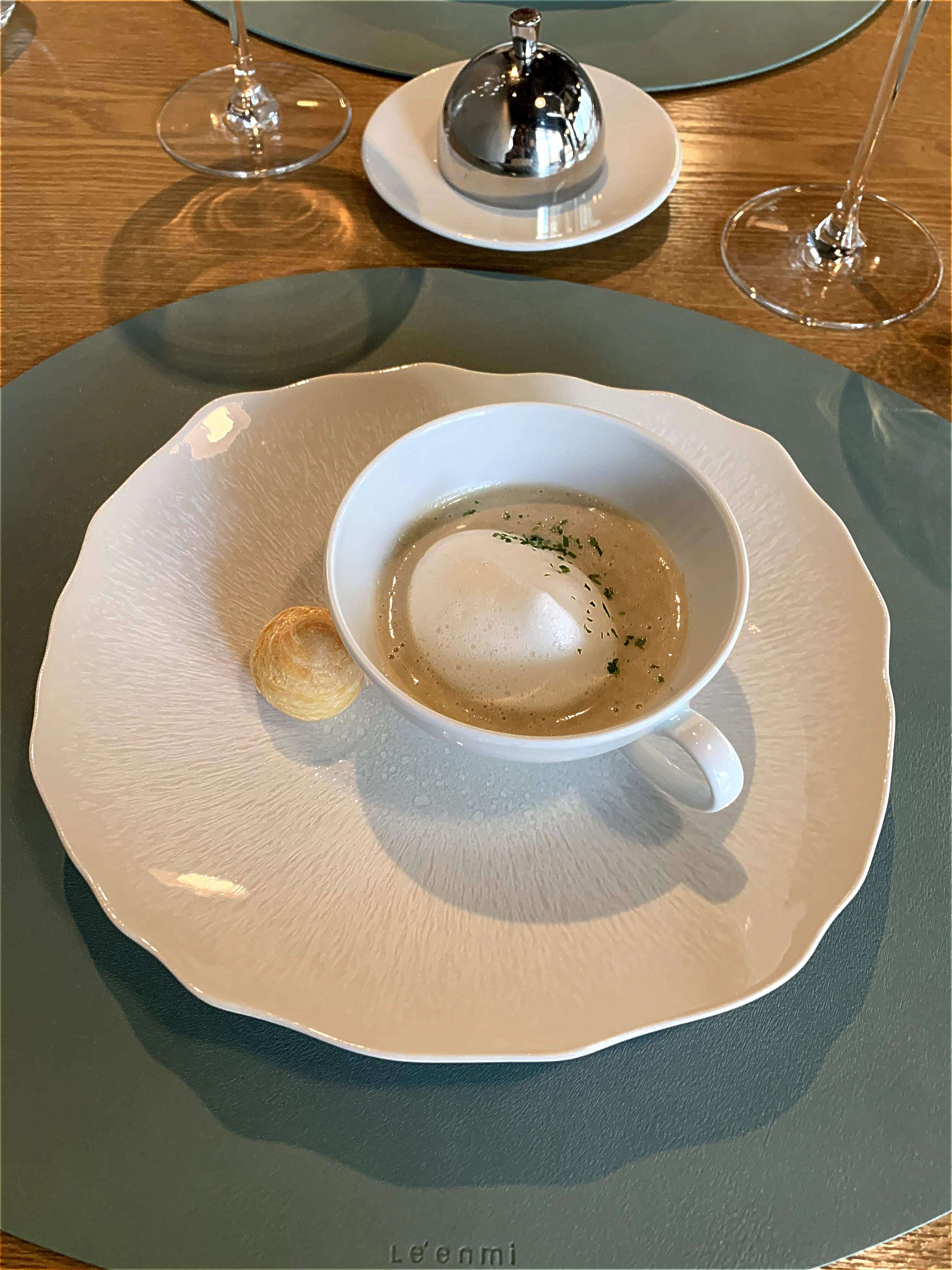
Sharp Soup is the name of the image that I will evaluate. Below is the original image then the blurred image and resharpened image:

The resharpened image is more sharpened than the original and resembles the sharpened version of the original more. Overall, however, most of the details that we can see in the original image but not in the blurred image, such as the texture of the pastry, have been preserved in the resharpened version. Overall, the resharpened version looks quite realistic and similar to the original.
The original Sharp Soup appears to be quite clear at first:
Although it was taken from an iPhone camera, we can see the bubbles in the foam on the soup, as well as the fine details in the plate.
However, once we sharpen the image using our unsharp mask filter, these high frequencies become much stronger and prominent, making the original image appear to be the one that was blurred.

We get a similar sharpened result when we blur the image first to find the high frequencies, instead of using the unsharp mask filter:
The following is not my image: credit goes to wallpapertip.com
Below is the sharpened version.
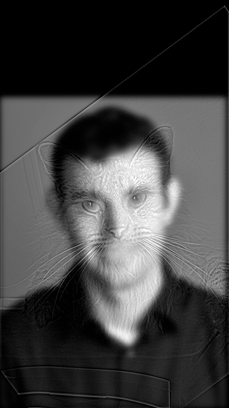
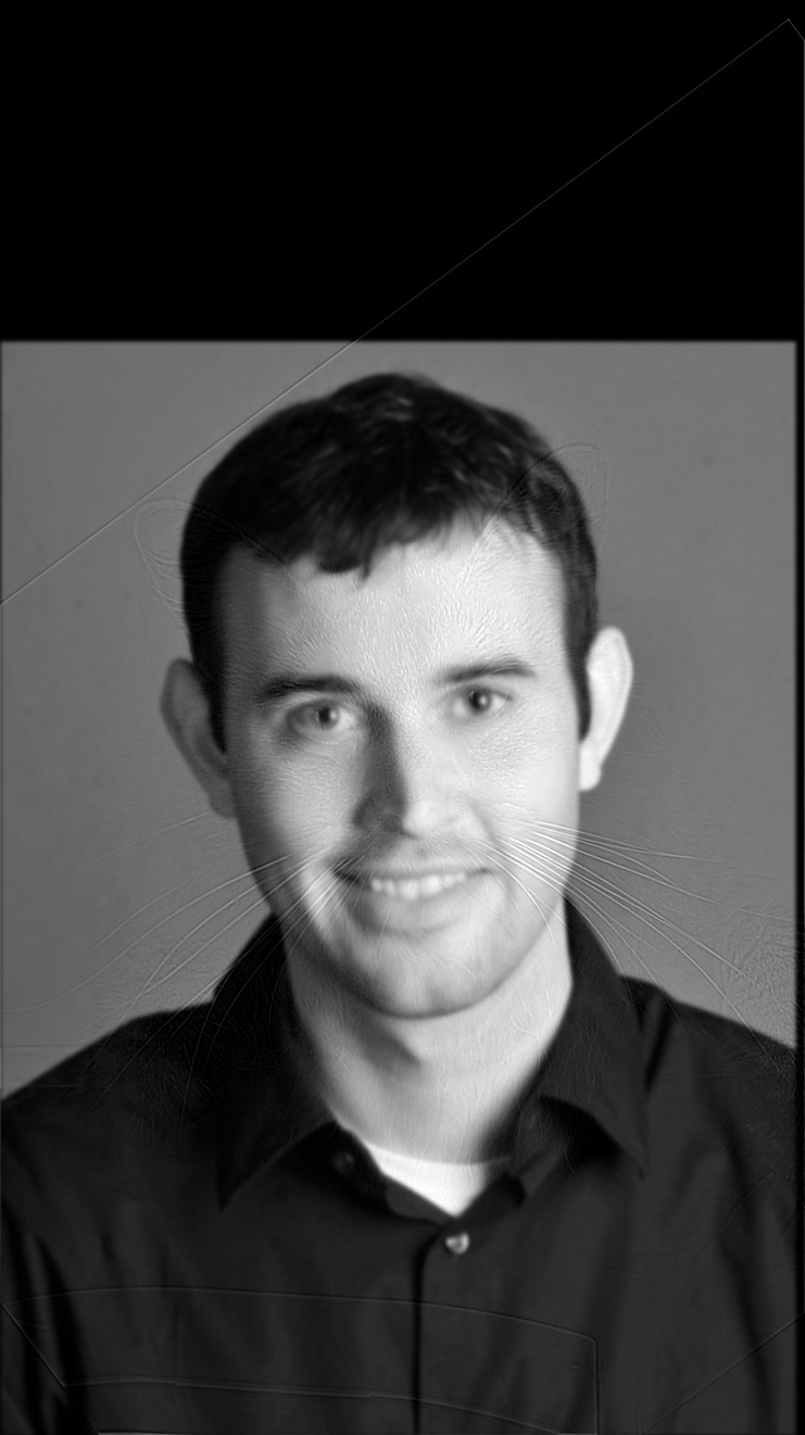
We now used the idea of representing pictures with different frequencies in order to create hybrid images. Below is the Derick-Nutmeg hybrid that my code created:
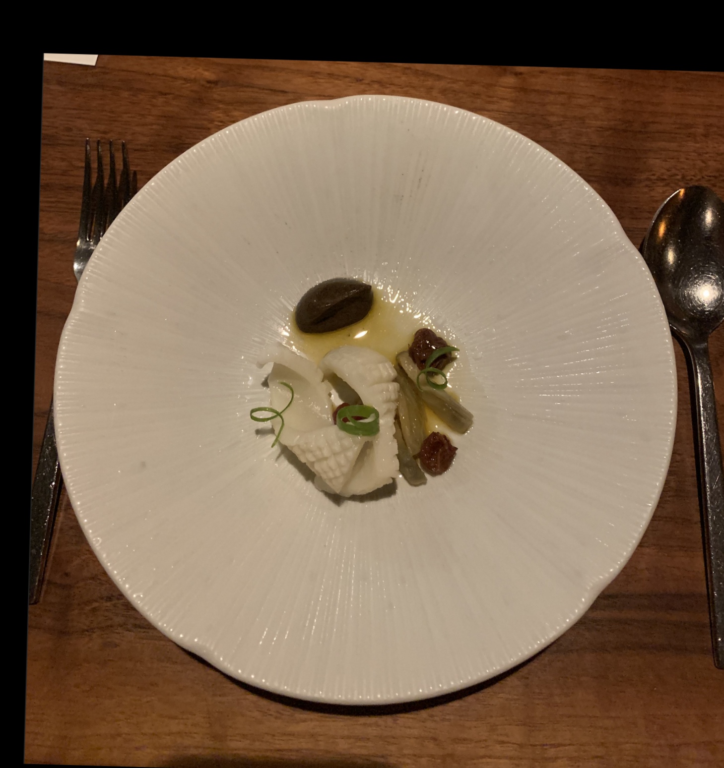
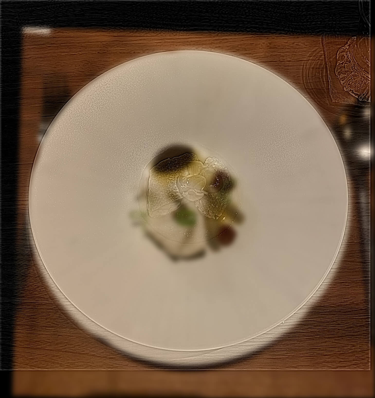
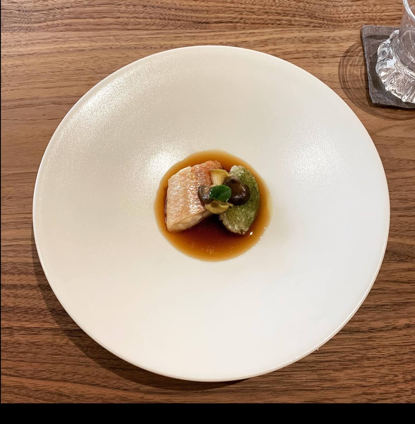
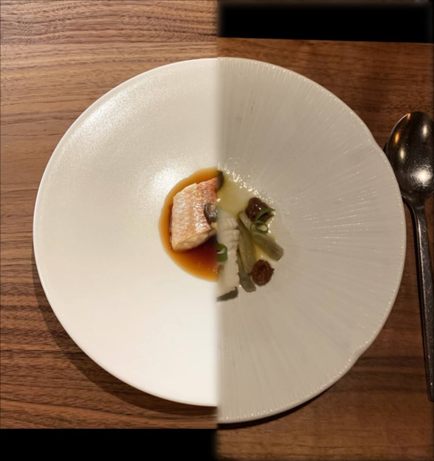
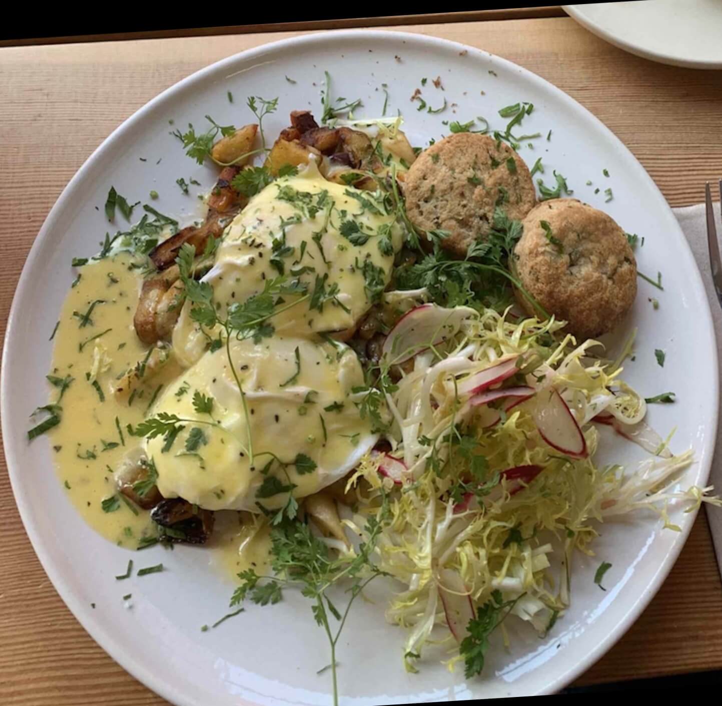
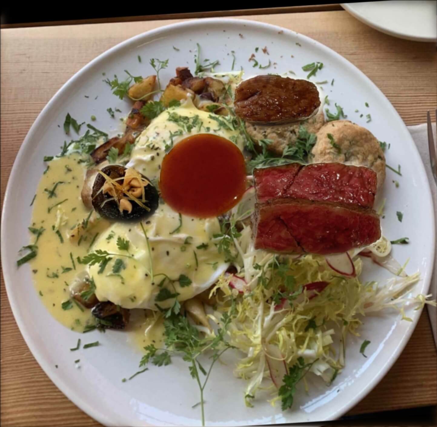
Below, I created a hybrid image of two seafood dishes I ate for dinner.
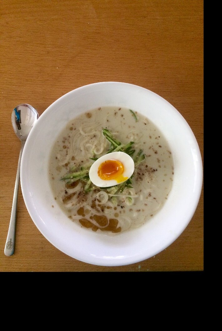
Dish 1:
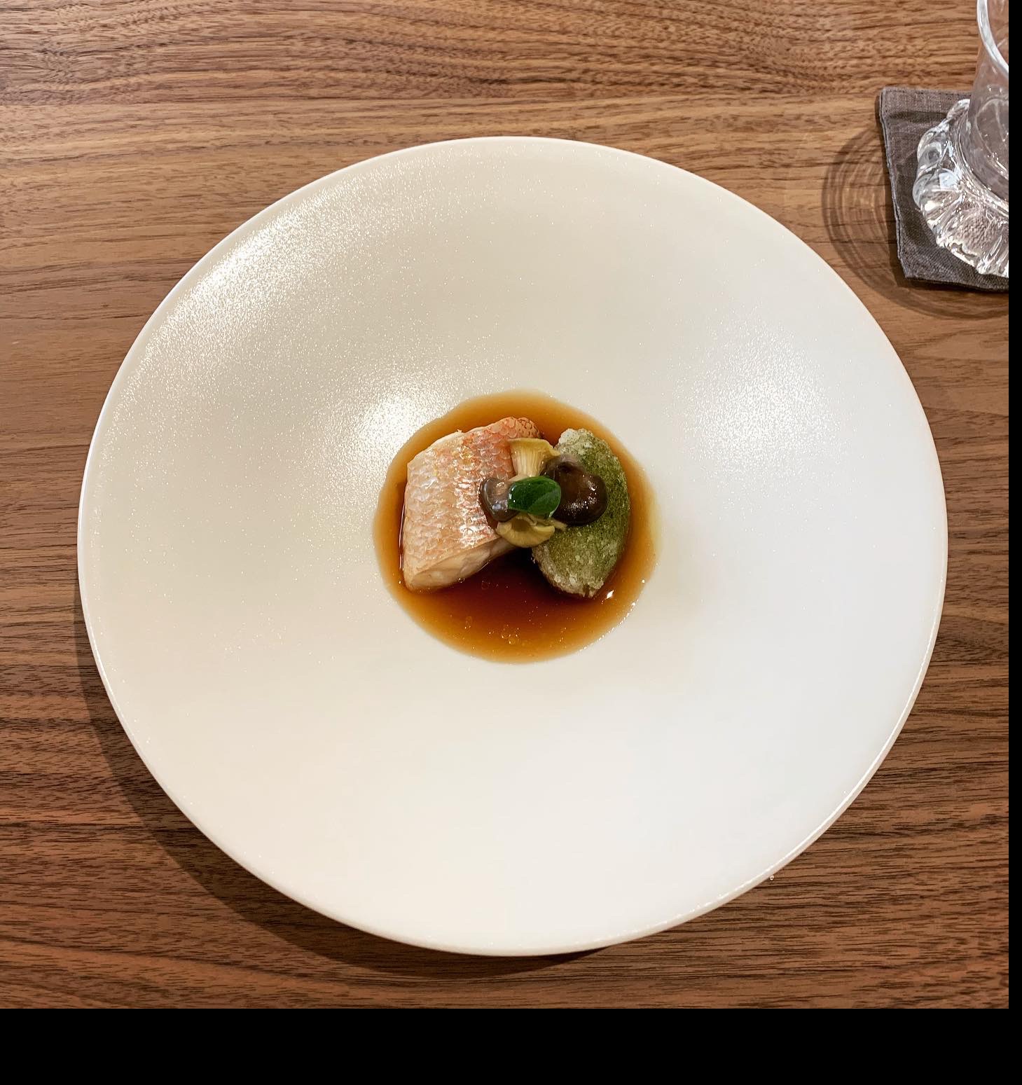
Dish 2:
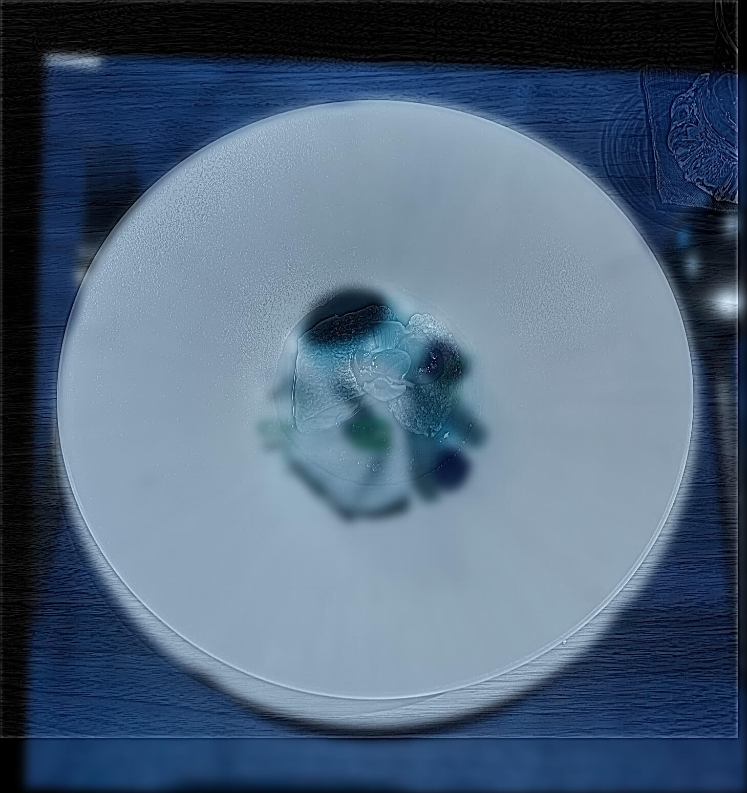
Hybridized Dish:
Here is the log FFT of the grayscale version (the value channel of the HSV version) of Dish 1:
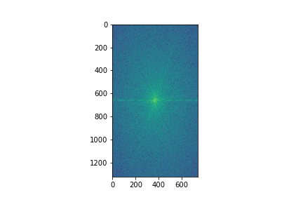
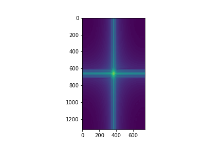
Here is the log FFT of the filtered version of Dish 1:
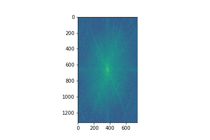
Here is the log FFT of the grayscale version (the value channel of the HSV version) of Dish 2:
Here is the log FFT of the filtered version of Dish 2:
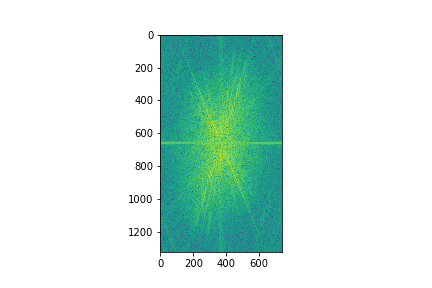
Here is the log FFT of the hybridized dishes:

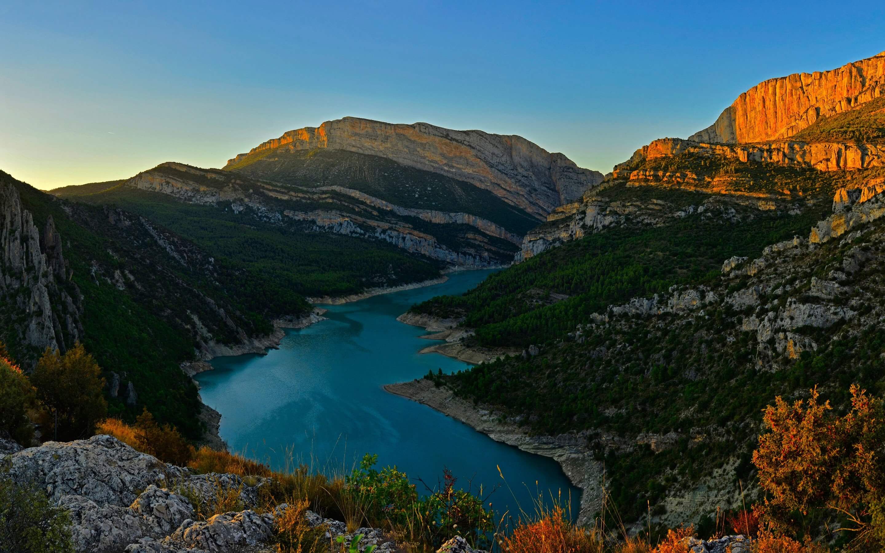
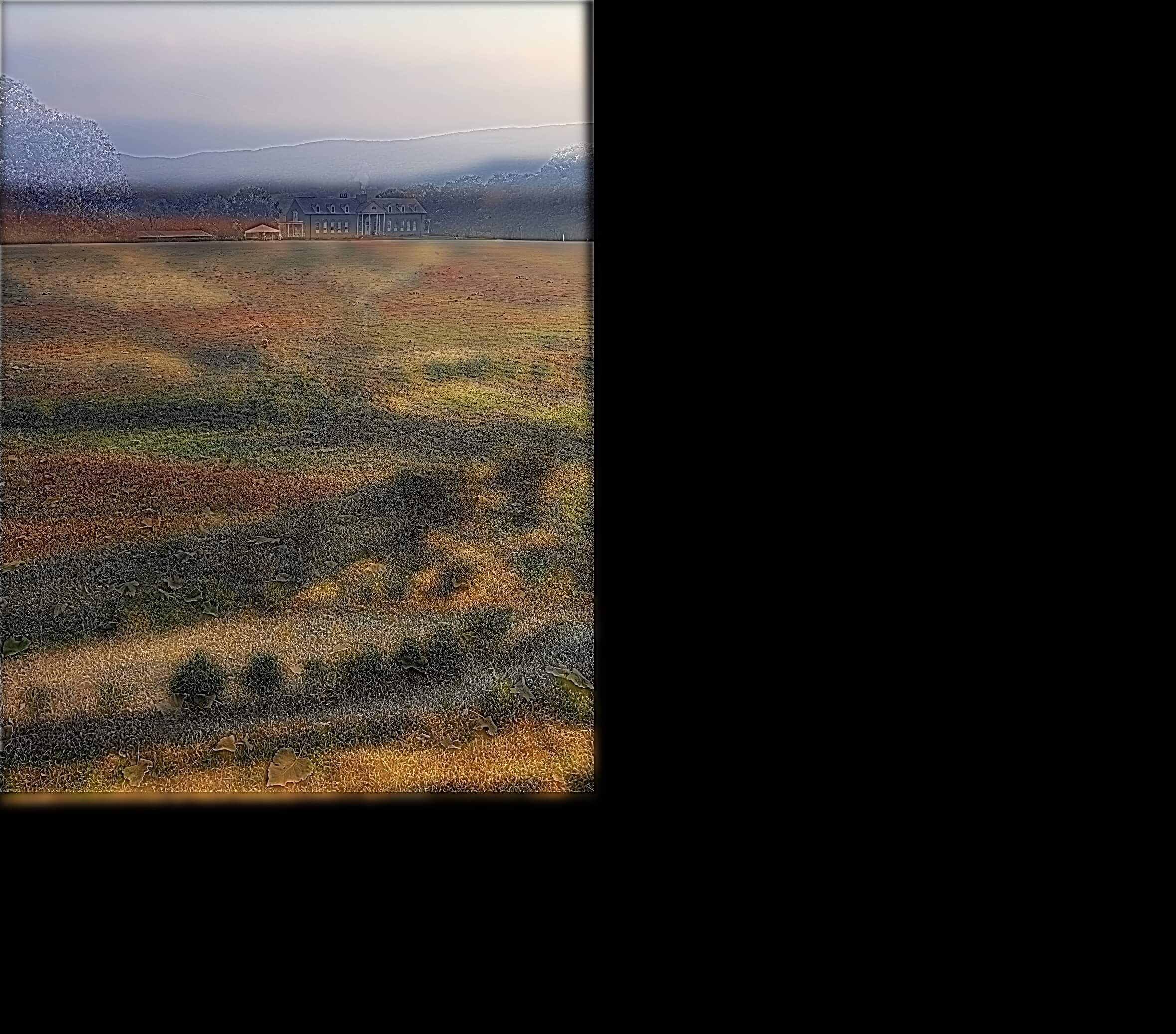
Here is a hybridized version of the landscape.
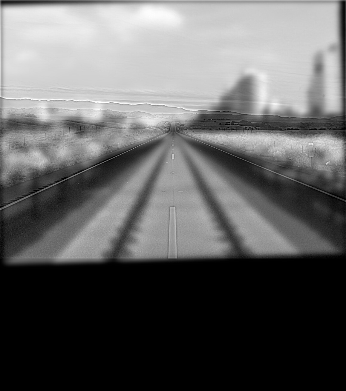
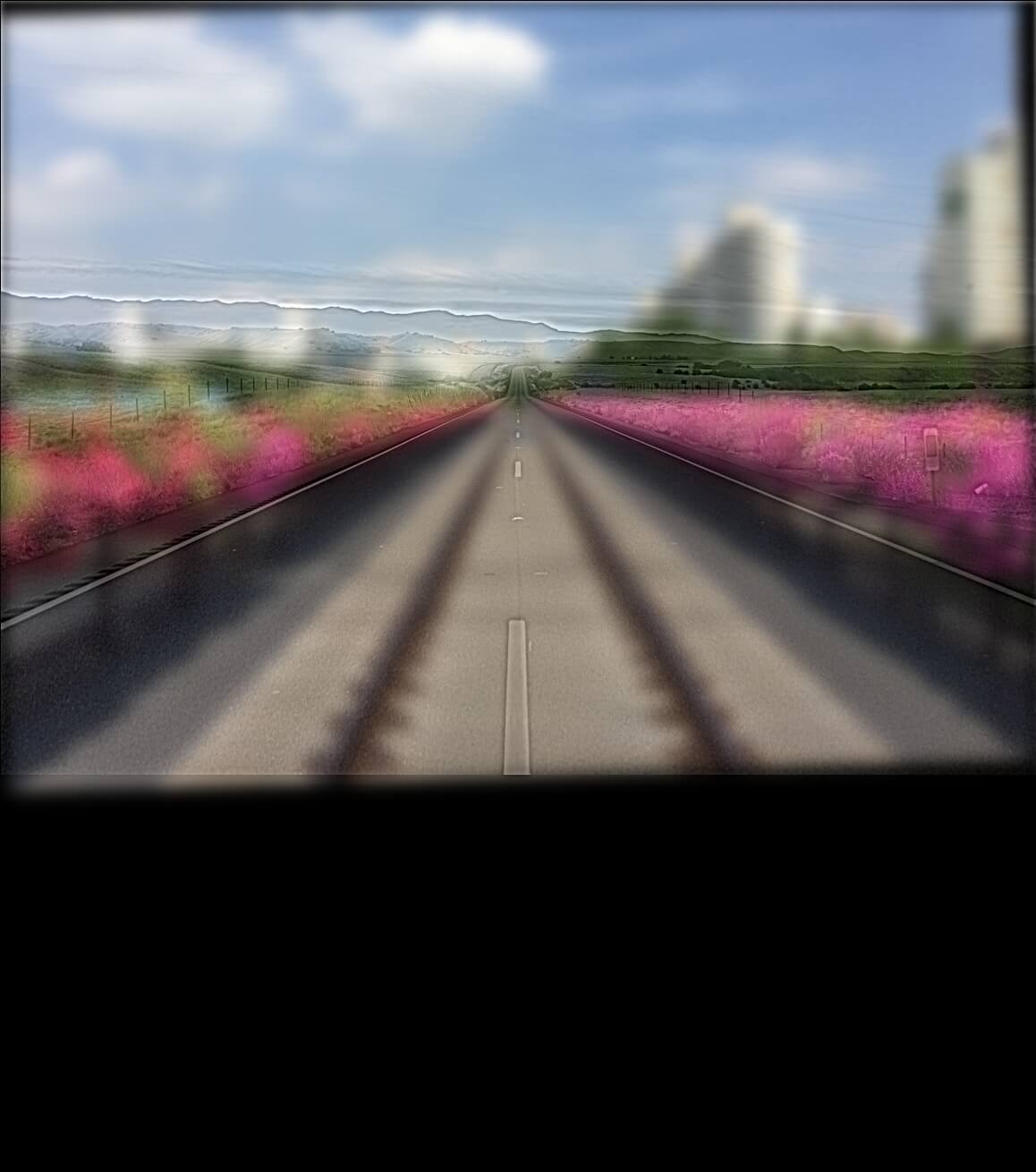
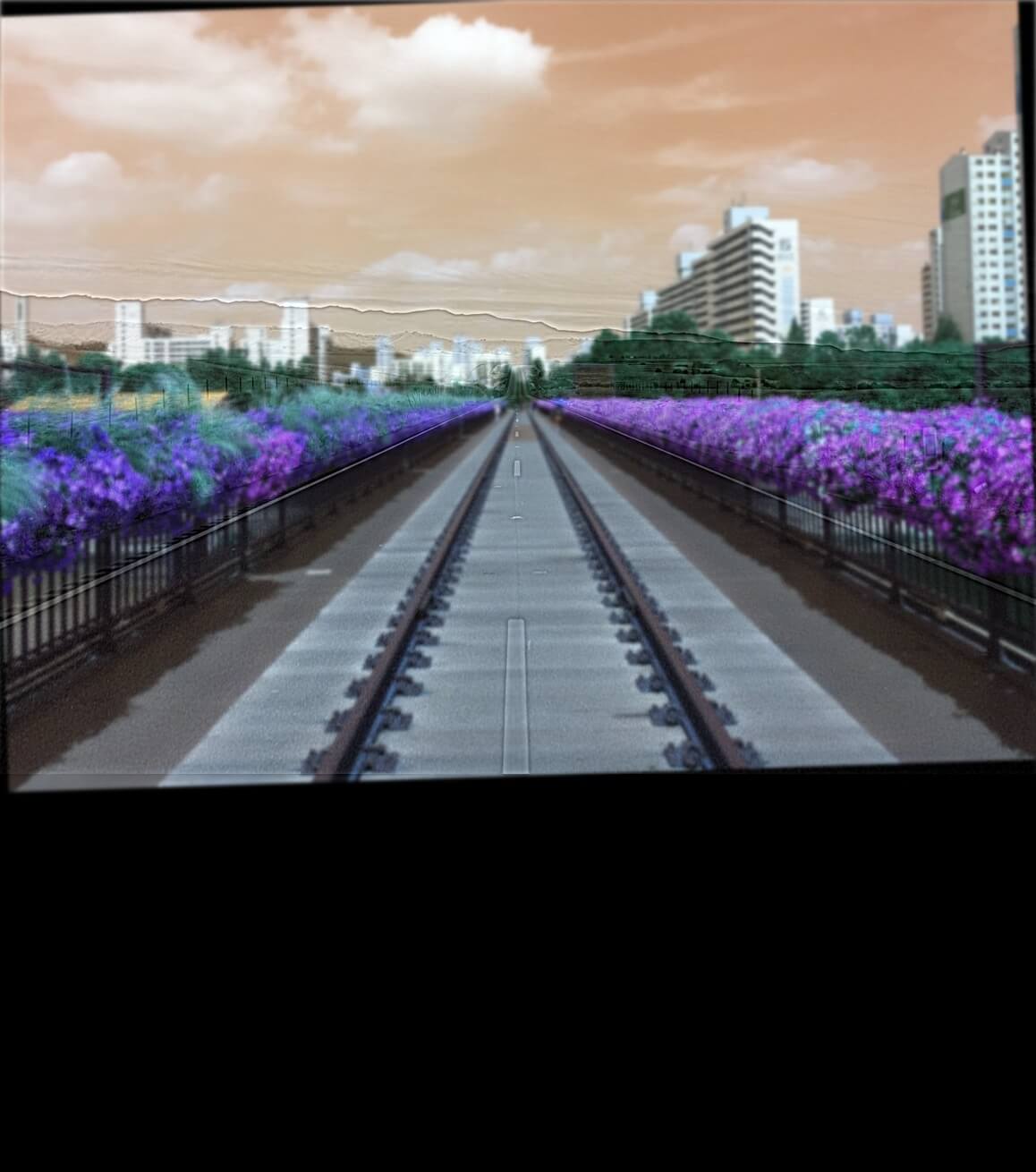
Here is a hybridized version of the road.

Before deciding what color configuration to do, I ran the sample hybrid images through four possible color configurations: both grayscale, high frequency grayscale, low frequency grayscale, and both color.
All color:
High gray:
Low gray:
All gray:

The high frequency image, even when colored, appears grayscale, so the hybrid image doesn't look very different even when both the low and high frequncies are colored. I decided to only color the low frequency image for this reason. Here are the colored hybrid images that I implemented for the bells and whistles section.
While tuning the parameters of the Gaussian filter and Laplacian filters, I ran into a few failures. The images below have very faint high frequncies and sometimes the wrong color channels. These failure, however, ultimately lead me to the parameters that I wanted from my images.
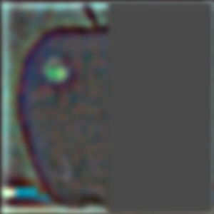
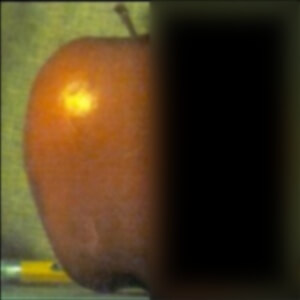
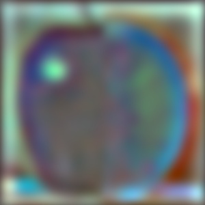
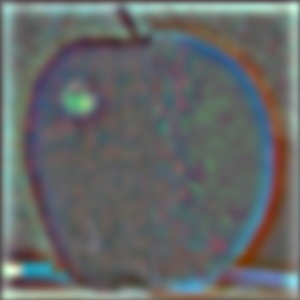
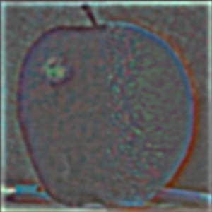
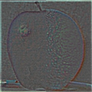
Apple level 1 to 4

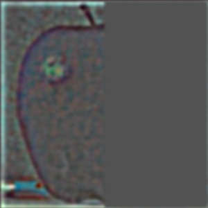
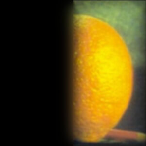
Orange Laplacian level 1 to 4


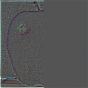
Orapple Laplacian level 1 to 4
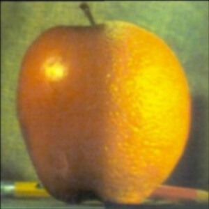
The final spliced image of the oraple:
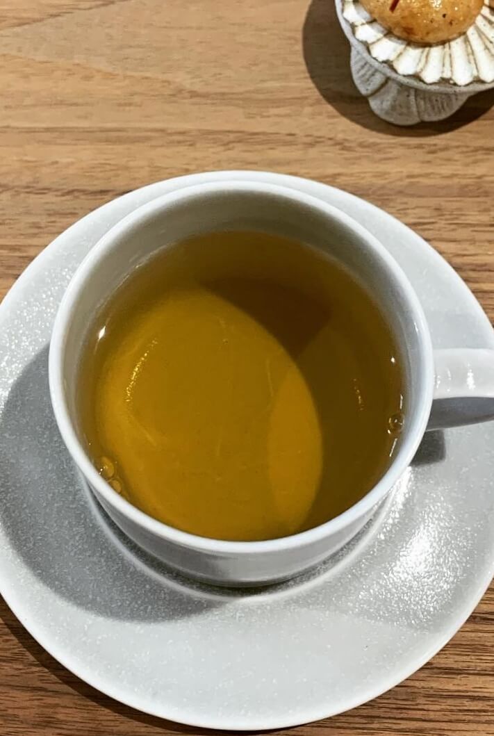
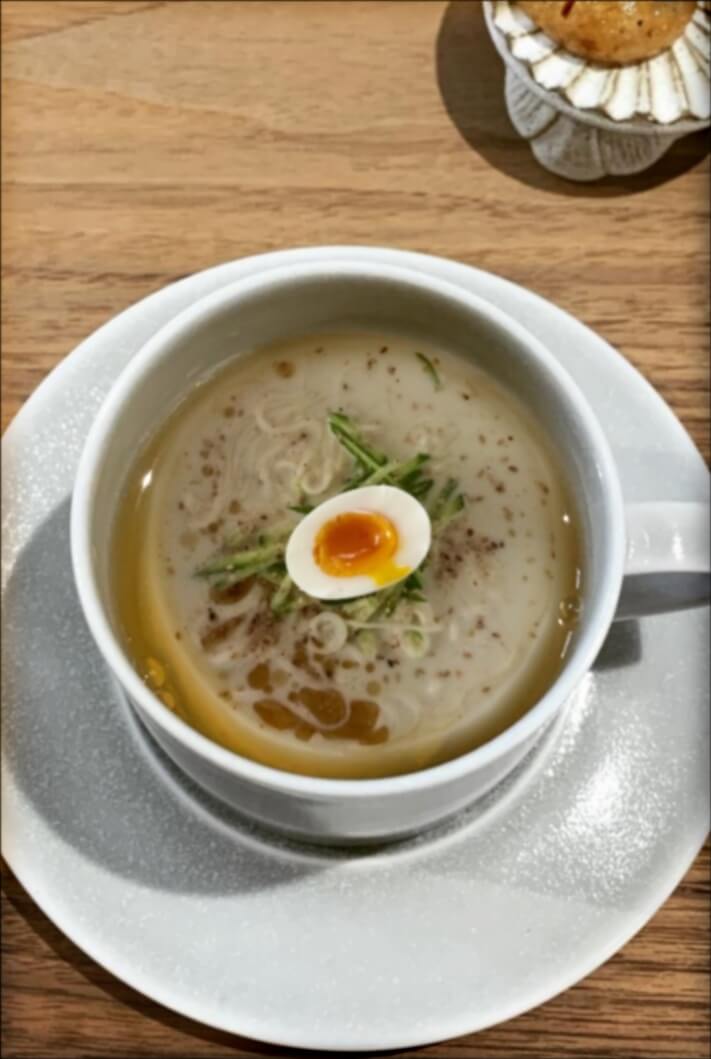
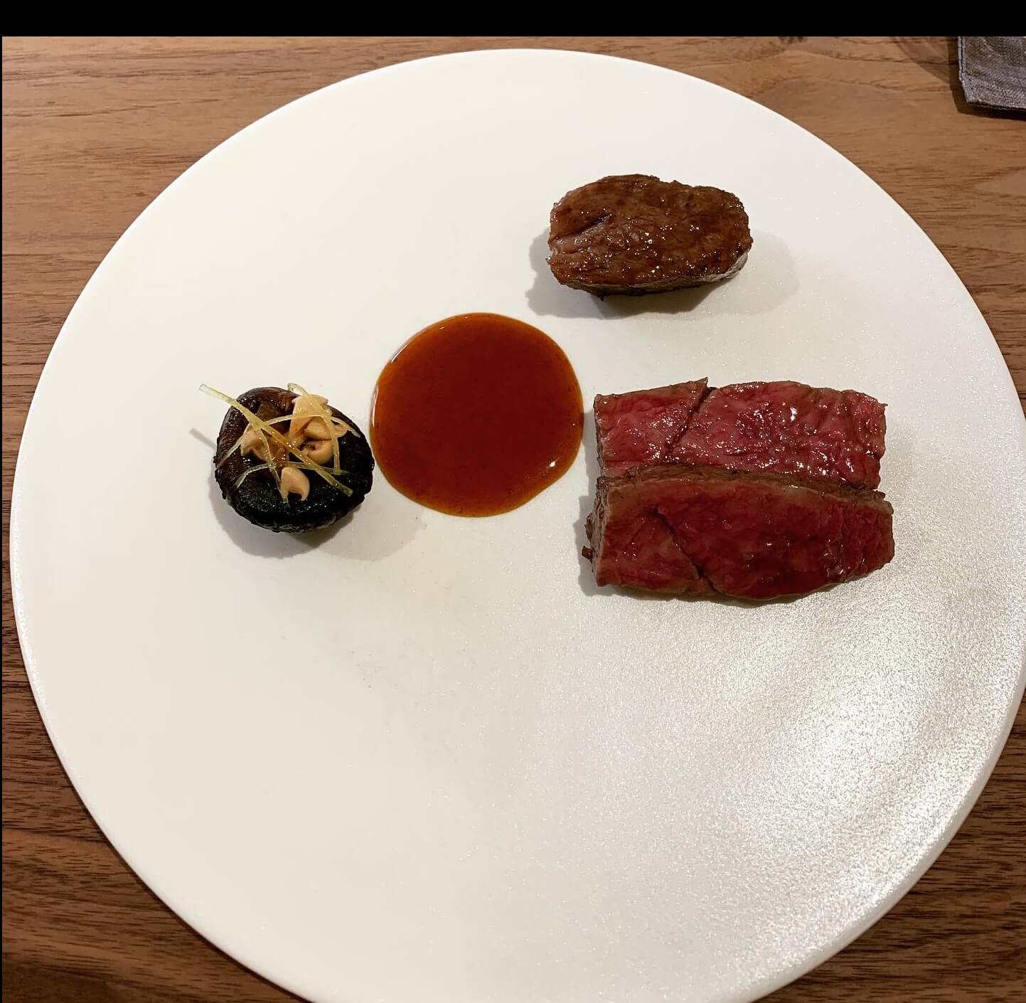
The dishes:
The soup in a teacup (Irregular):
The meaty salad (Irregular):
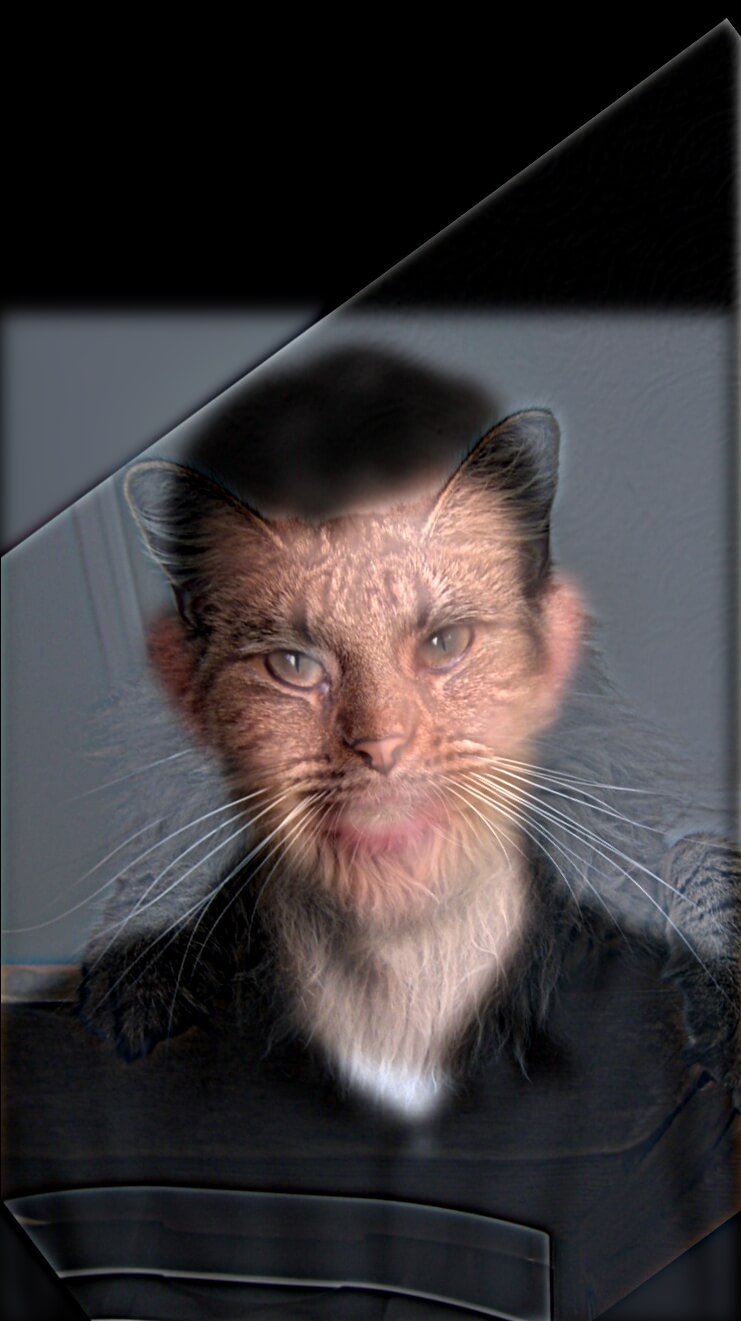
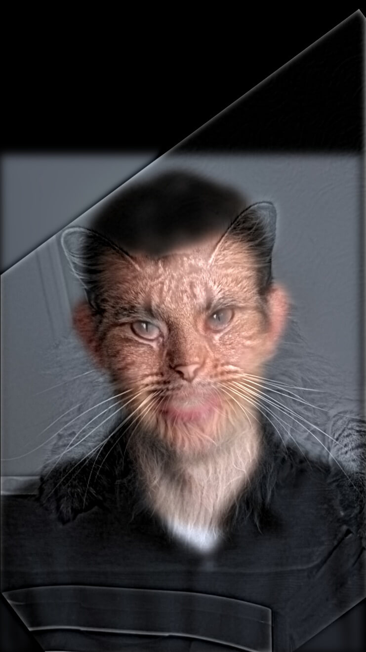
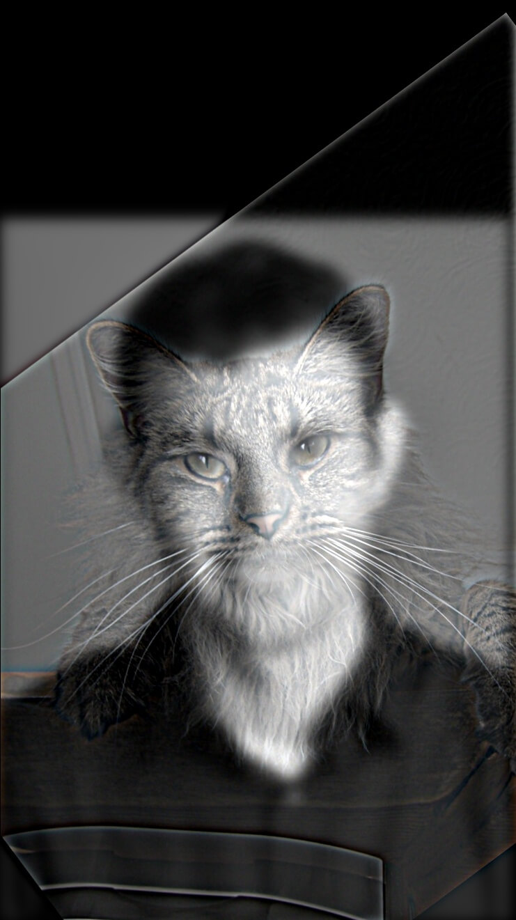
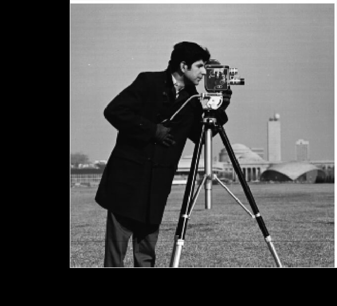
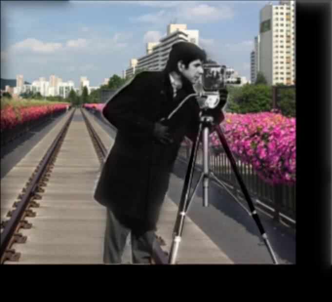
The cameraman in the road (Irregular):
The most interesting thing I have done in this project was splicing images into each other: I thought that it was really interesting how we were able to do this mechanically, especially since most of what I know about images is related to machine learning. I really enjoyed figuring out what images to hybridize with each other and splice into each other: it was a lot of fun to determine that would be compatible and interesting.