Arjun's CS294-26 Proj2
Part 1.1 Finite Difference Operator
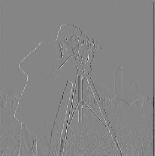
Cameraman dX (detects vertical edges). All the images in part 1 I linearly normalized for display such that the minimum value is 0 and the maximum is 1
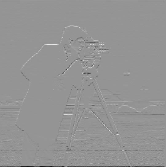
Cameraman dY (detects horizontal edges)
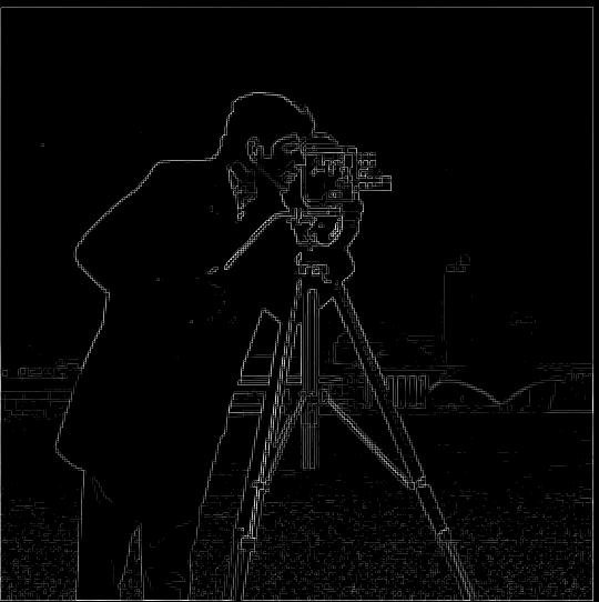
Cameraman Edges (norm of [dX, dY] > Thresh). I used a threshold of 3 times the mean norm.
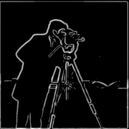
Part 1.2 Derivative of Gaussian Filter
Cameraman, first gaussian blur then edge convolution

Cameraman, single convolution gaussian and edge.
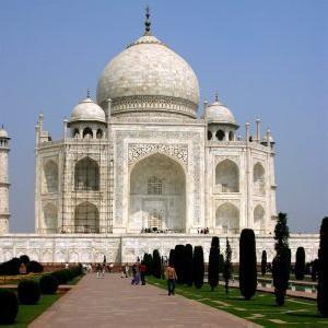
Part 2.1 Image Sharpening
Taj, alpha=0.0, 0.5, 1.0, 2.0. I think the best value is probably between 0.5 and 1.0. More than that these unnatural halos form, and less than that it's a little blury.


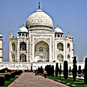
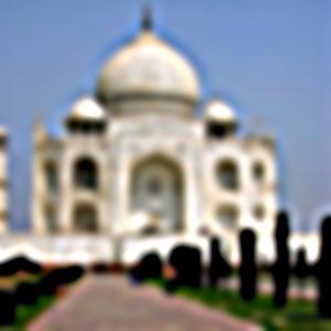
Blurring Taj alpha=2.0 then sharpening again with the same alpha yields the below image. Its a lot more blurry then the original alpha=2.0 since our sharpening can only highlight high frequency signal that's already there. The blurring step permanently removes much that.
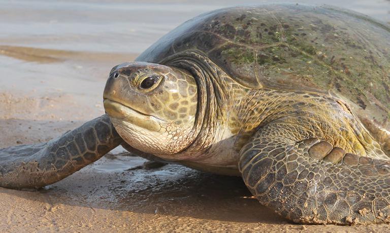
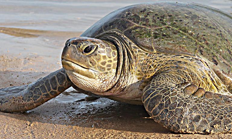
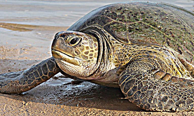
My image #1 Turtle, same values of alpha. Here I think a greater alpha such as between 1.0 to 2.0 actually works best. I suppose that's because the original was a little more blurry. In general sharpening makes this one a lot better.

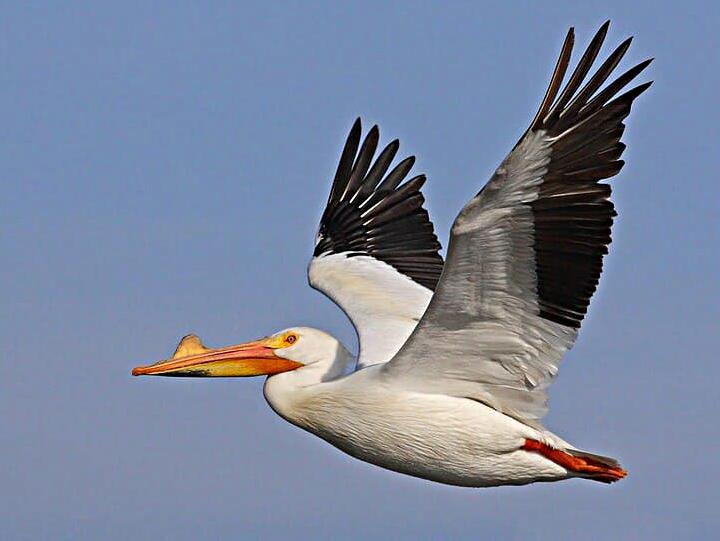
My image #2 Pelican, same values of alpha. Sharpening doesn't really help this one since unlike turtle, pelican is made up of much more low frequency color.


Part 2.2 Hybrid Images
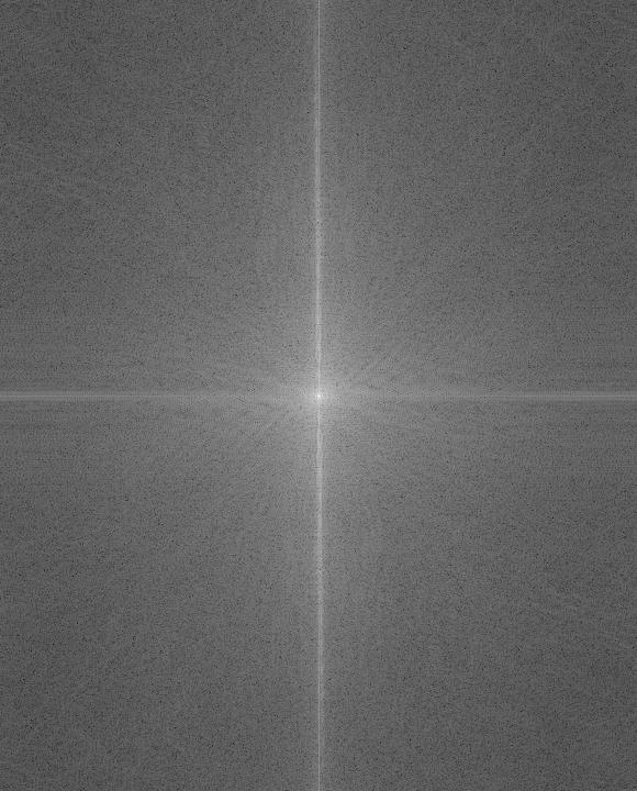
Frown (Left: Spatial, Right: Frequency)
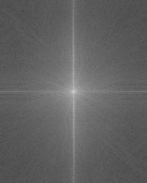
Smile (Left: Spatial, Right: Frequency)
Hybrid Image Frequency. Frown Low Pass ; Smile High Pass ; Sum of preceeding two.
You can clearly see how the off axis high frequency components are tempered in the low pass.
I suppose the on axis components are so strong that they continue to remain somewhat present.
For the high pass you can see how right around the origin the strength is low as we've eliminated
those frequencies.
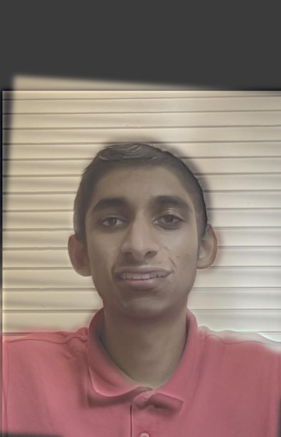
Frown-Smile: The two below are resizings of the same image! Since we kept the smile high frequencies
that's what stands out up close. Away those are too small to see and the originally low frequency frown
enters are target frequency range.
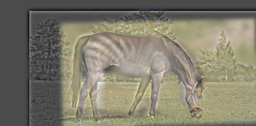
Zebra and Horse (I managed to find a pair in similar poses!)
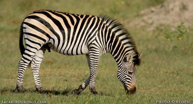
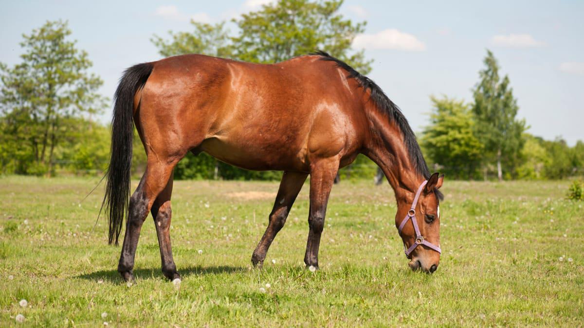
Zebra-Horse: similar phenomenon as before (Zebra low pass + Horse high pass). Interesting note here is that Zebra-Horse worked a lot better than Horse-Zebra due to Zebra's natural high frequency stripes.
Part 2.3 Gaussian and Laplacian Stacks
We demonstrate the gaussian and laplacian stack on the oraple as suggested.
Here we have a gaussian stack of depth 4.


And the differences become the laplacian stack of depth 4.
Part 2.4 Multiresolution Blending
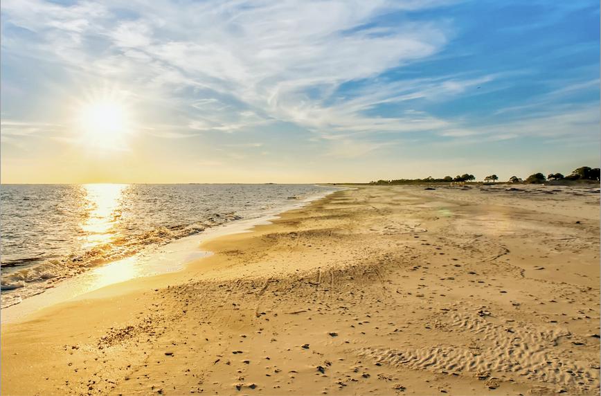
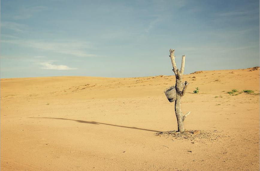
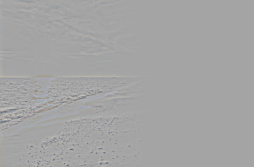
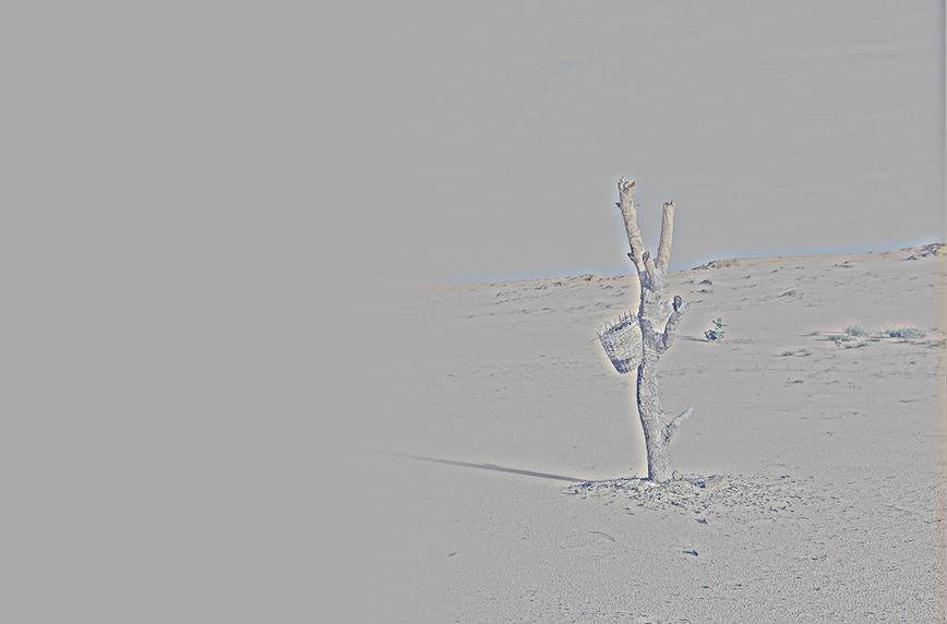
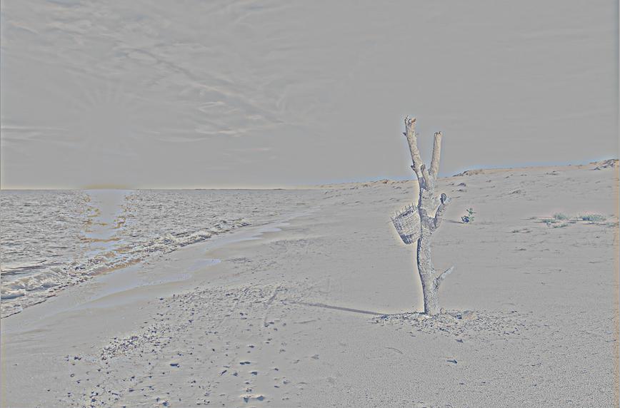
First I blended a beach and dessert scene. Critical for successful blending here was to use a smooth initial mask rather than the suggested step function. I additionally implemented a gaussian/laplacian pryramid for this part since that allowed me to apply far larger effective gaussians in the same computational time. First we see the original images and mask. The mask is just a gaussian blurred edge.

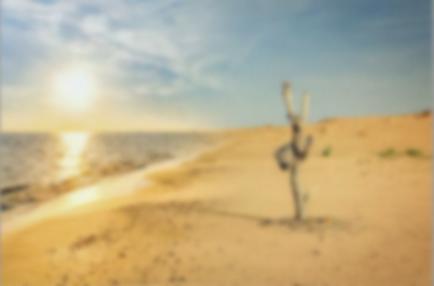
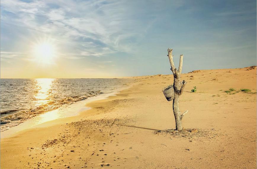
And the blended result, following the paper! To get a result as smooth as this, I manually alligned the skylines of the original images. (Using the provided alignment script left some undesirable artifacts.)

To illustrate the process we show all the components that go into this blending. Starting with the last level of the gaussian pyramids weighted contributions then going all the way down the laplacian pyramid.
For completeness we also show the state of the aggregated image which continually gets refined till it reaches the end result.


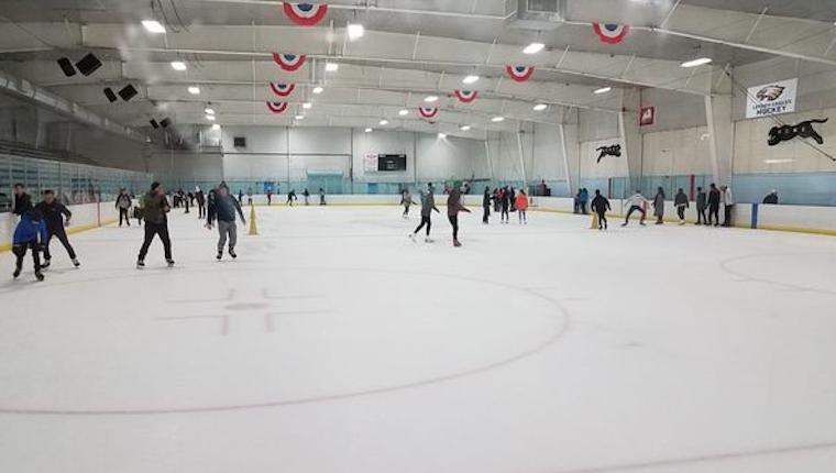
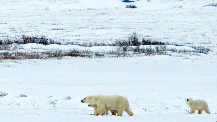
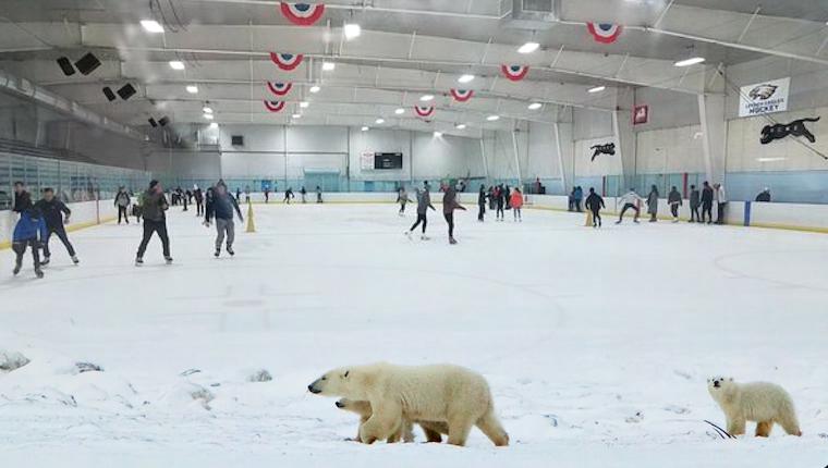
Next we blend an icerink with artic scene including a couple polar bears. Similar to the previous example I chose a pair that worked well together, meaning the seam area has roughly similar colors.

And again the blended result!
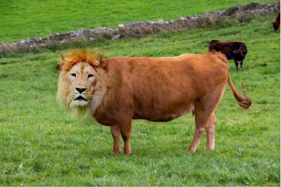
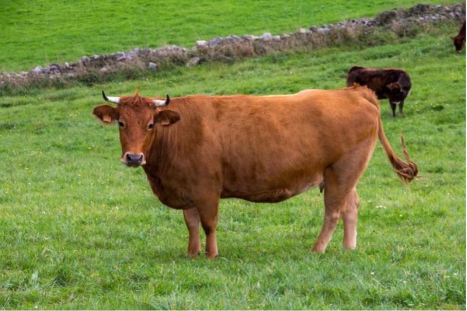
As an irregular mask we consider imposing the face of a lion onto the body of a cow.

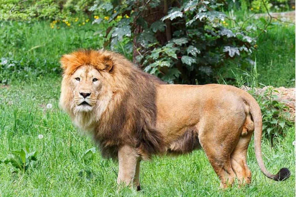
And again the blended result!