In this project we learned about different ways in which to manipulate images using filters and a rudimentary understanding of frequencies. Using finite difference operators, we were able to construct partial derivative images with respect to x and y which were then used to produce a gradient magnitude image which was very good at detecting edges. To reduce noise we applied a gaussian (low-pass) filter to remove some of the higher frequencies from the image that were causing the noise.
The gaussian filter is a very good and nice low pass filter which can be used to remove high frequencies within an image. Likewise, subtracting a low-pass filtered version of an image from its original will reveal the high frequencies of the image. We can use these tricks to create a Laplacian filter which retains the high frequencies of the image while discarding the low frequencies (high-pass filter). These filters can be used for image sharpening, hybrid image creation, or more elaborately in gaussian and Laplacian stacks which are then used to perform multiresolution blending of two images given a mask which significantly smooths out the boundary between the two images. The following report will go into more detail about the algorithms and implementations of each of these features using filters and frequencies for image manipulation.
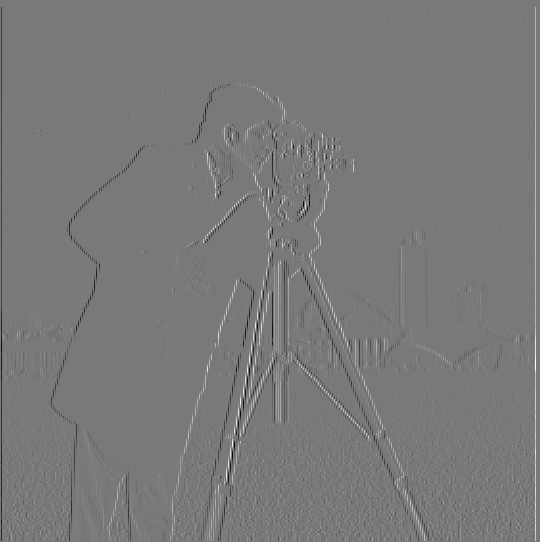
One of the fundamental ways to identify edges in an image is to use finite difference operators. The finite difference operators used in this project were the following:
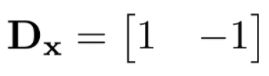
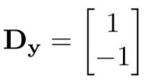
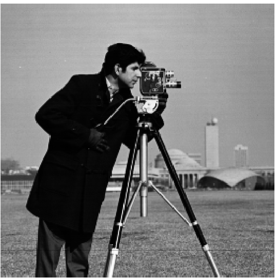
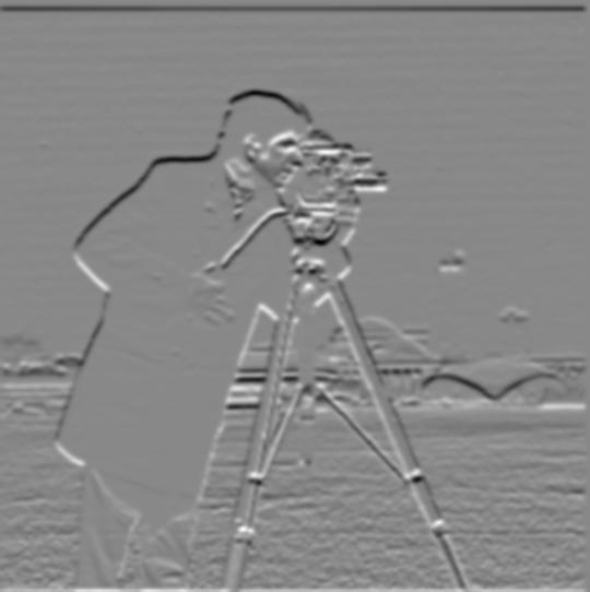
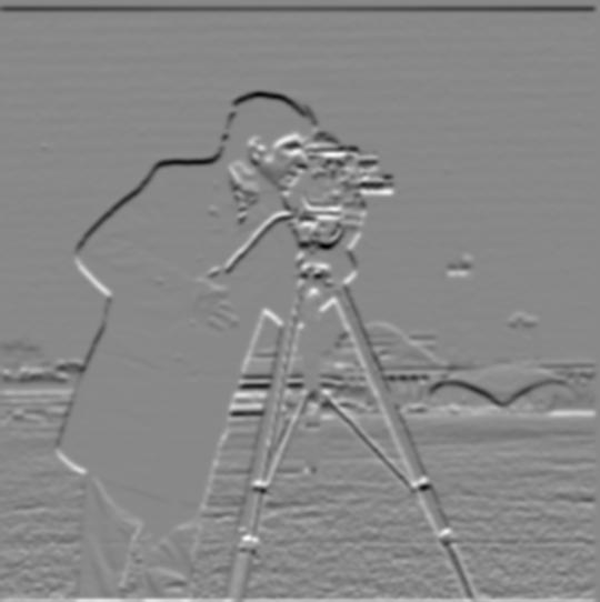
We can use these finite difference operators in a convolution with an image in order to get the partial derivates of the image with respect to x and y. In this example, by convolving the cameraman image with the Dx finite difference operator, we can get the partial derivative of the image with respect to x. Likewise, by convolving the cameraman image with the Dy finite difference operator, we can get the partial derivative of the image with respect to y. Visually inspecting the outputted partial derivative images it is apparent that the finite difference operators highlight boundaries in the image that we perceive as sharp edges, or a quick change in pixel values relative to adjacent pixels. You can view the original cameraman image along with its x and y partial derivative images below:
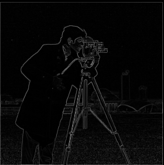
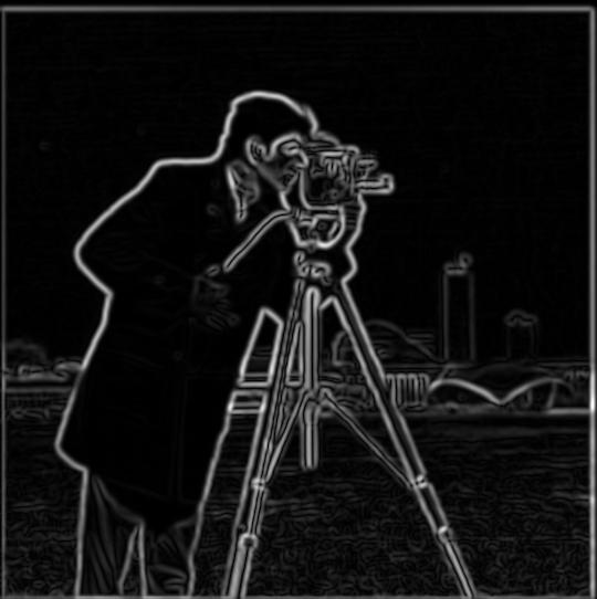
In order to better visualize the edges present in the image we can compute the gradient magnitude of the cameraman image from the x and y partial derivative images. In essence, the gradient magnitude is an edge detection algorithm that can be computed by first squaring all the pixel values in both the x and y partial derivative images, then summing the x derivative squared image values with the y derivative squared image values, and lastly by taking the square root of each pixel value in the sum. If dx represents the x partial derivative image and dy represents the y partial derivative image, then the gradient magnitude of the cameraman image is defined as follows:

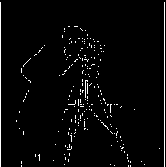
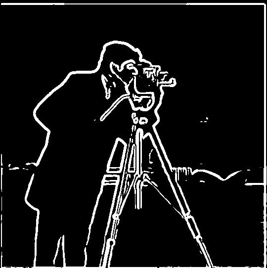
The gradient magnitude of the cameraman image is viewable below along with a modified gradient magnitude image on which a threshold was applied to make the edges more visible. The threshold simply compares each pixel value to a specified threshold value and if the pixel value falls below the threshold, then the pixel value is set to 0 and if the pixel value is at least as great as the threshold, the pixel value is set to 1. This allows for the gradient magnitude image to consists of high contrast black and white pixels rather than gray pixels which make it a bit harder to see the edges.
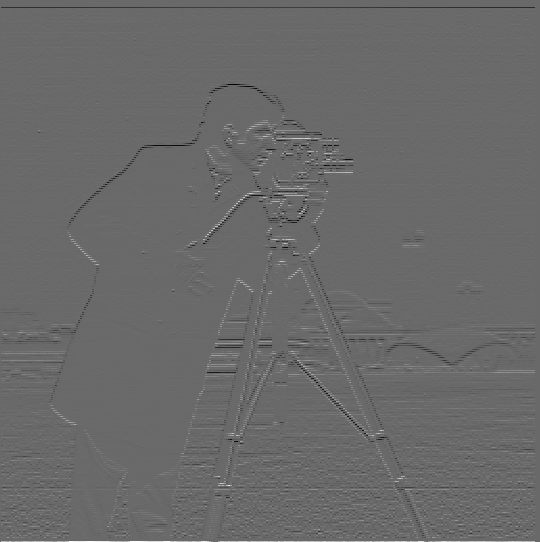
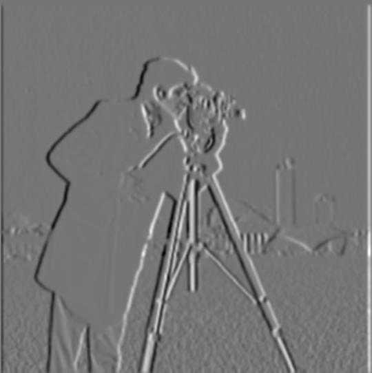
From Part 1.1, we observe that the edges detected by the gradient magnitude algorithm can be noisy. In this section, we attempt to remove some of the noise from the edges by applying a gaussian filter on the cameraman image. The noise in the edges depicted in the previous subpart indicates that the image has some very high frequencies which are being picked-up by the finite difference operators. We can remove the noise by low-pass filtering the image with the gaussian filter which will remove the higher frequencies in the image. The greater the value of sigma (and correspondingly the kernel width of the gaussian filter) the more the image will become blurred and higher frequencies removed from the original image. The output of the blurred cameraman image and its partial derivative images can be viewed below:


Likewise, we can use the partial derivative images produced from the blurred cameraman image to create the gradient magnitude for the low-pass filtered image with the results viewable below:
We can immediately observe that the low-pass filtered image has much thicker edges in the gradient magnitude image which are also more discernable visually. Intuitively, prior to low-pass filtering the image, the noisy edges we observed in the gradient magnitude image were the result of very high frequencies in the image, or a rapid change in pixel value that may only last for one pixel, hence the noisy results. By applying a gaussian blur on the image first, low-pass filtering the image, we remove some of those very high frequencies in the image so that what previously was observed as a single pixel value that had a drastically different pixel value from its adjacent pixels would be smoothed out to several pixels with not as abrupt of a pixel value change. This is the underlying mechanism of low-pass filtering and the reason why the edges are thicker and more defined in the low-pass filtered gradient magnitude image. Thus, applying a gaussian filter to the image achieved the result of denoising the edges detected by the gradient magnitude.
As instructed, we further simplified this process of blurring the image before computing its gradient magnitude by creating a derivative of gaussian (DoG) filter which was made by first convolving the gaussian filter with each finite difference operator. Then a single convolution can be used for computing the partial derivative with respect to x and y images. The results of using the DoG filter can be viewed below and as expected yield the same output.


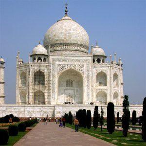
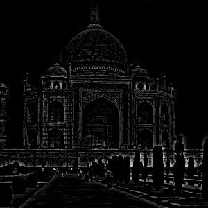
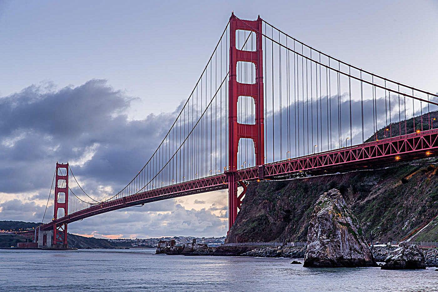
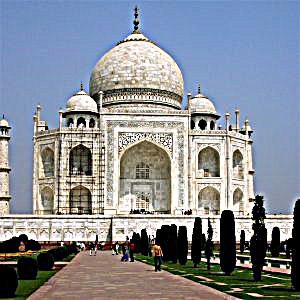
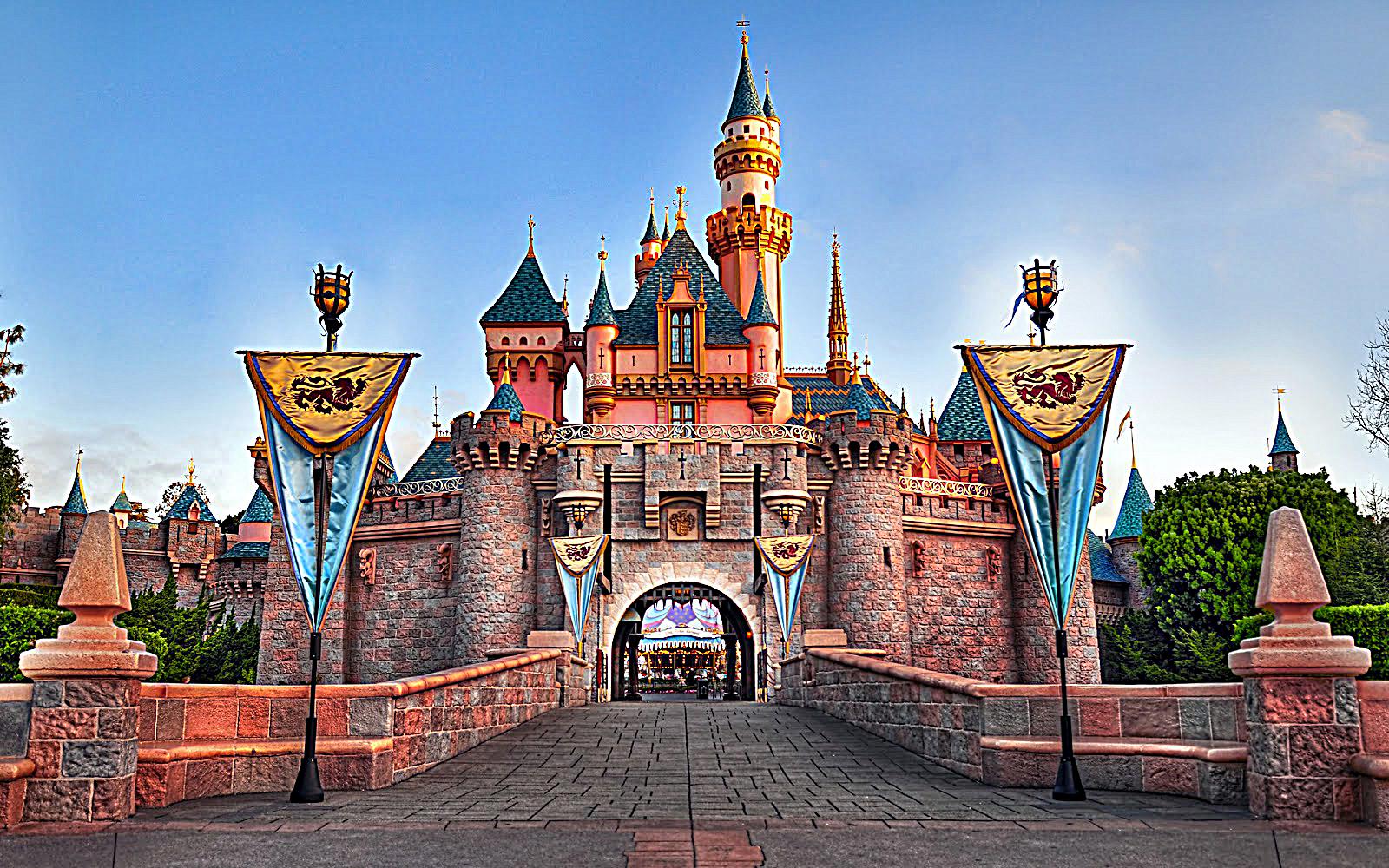
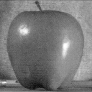
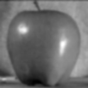
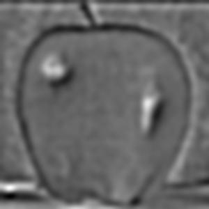
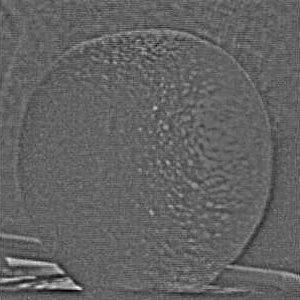
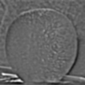
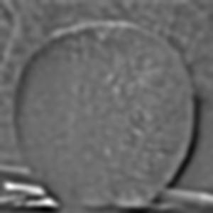
In this section, we sharpen images by increasing the high frequencies already present in the image. Intuitively, from the previous part of this project, we observed that a gaussian filter can be used as a low-pass filter to remove the high frequencies from an image. Taking the image after it has been low-passed and subtracting its values from the original image would then yield the high frequencies in the original image, since we subtracted away the low frequencies from the low-pass filtered image. From the resulting high-frequency image, we can then apply a magnitude scalar and add those scaled high frequencies to the original image, which will result in perceives sharpening of edges. The images below show the original image, the low-pass filtered image, the high-frequency image, and the sharpened image with alpha = 1 for three different images. Taj.jpg was provided with the project files, castle.jpg was sourced online from castle source and bridge.jpg was sourced online from bridge source.

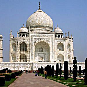

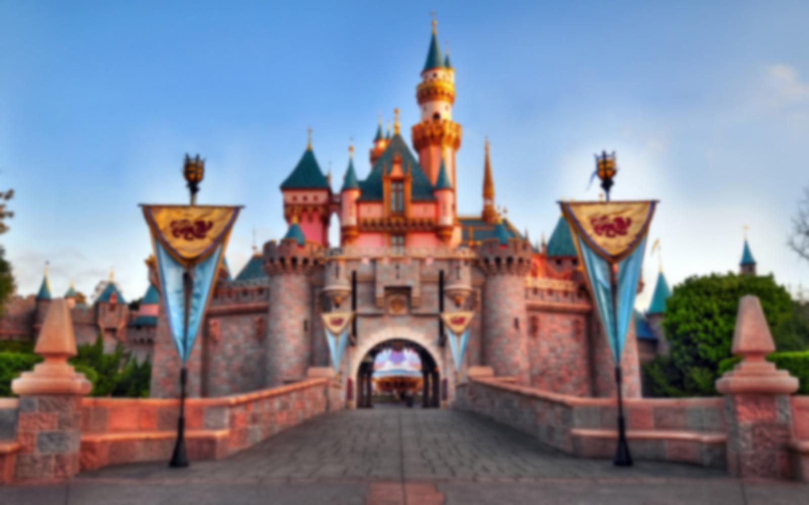

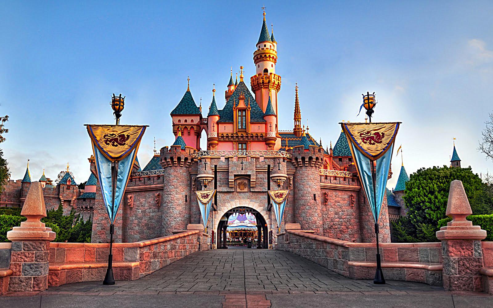

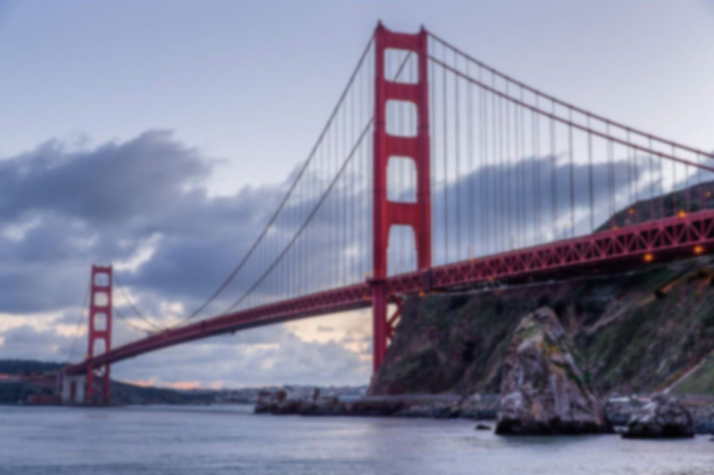
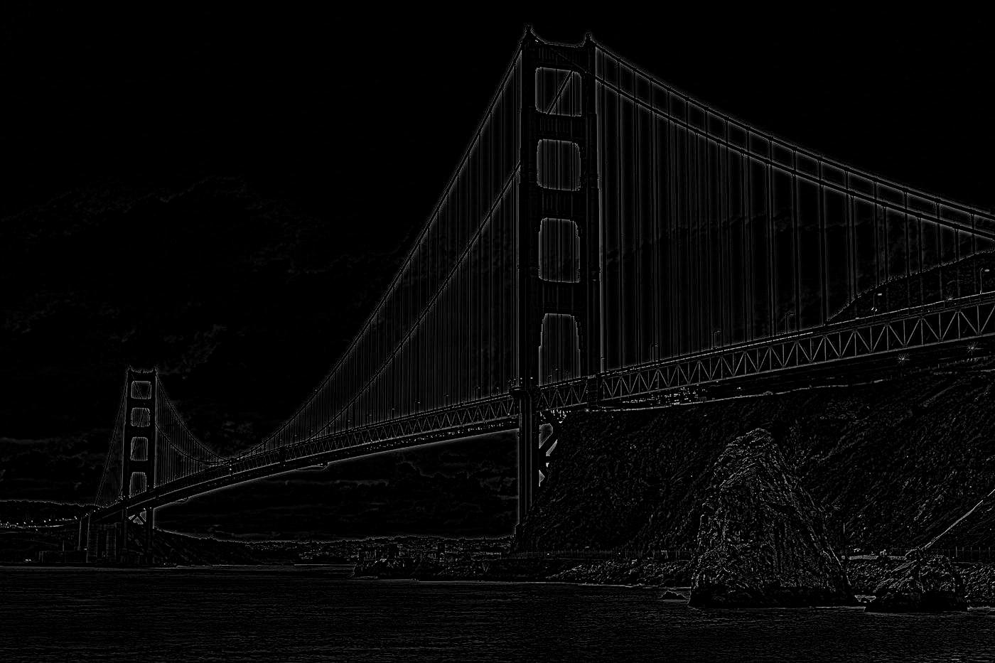
The intuitive idea of adding high frequencies to an image that was just explained above can be combined into a single convolution using an unsharp mask filter. To create the unsharp mask filter kernel with which to convolve the original image we first define an alpha term which is defined as the scalar magnitude with which to scale the high frequencies in the image (or how much sharpening you want in the image). From there, we define a unit impulse kernel of the same dimensions to be used with the gaussian filter in order to make the subtraction operation later on convenient. The unit impulse kernel is essential the identity of a convolution kernel, it just returns one pixel value. Likewise, we define the gaussian kernel to be used to low-pass the image. The unit impulse kernel is multiplied by (1 + alpha) and the gaussian kernel is multiplied by alpha. After both the unit impulse and gaussian kernels have been scaled, we subtract the scaled gaussian kernel from the scaled unit impulse kernel to produce the unsharp mask kernel. This will serve as our unsharp mask filter which, given an alpha and defined gaussian parameters, will sharpen our image in a single convolution. The unsharp mask filter is applied to each color channel of the color image prior to restacking to produce the sharpened color image. Below are the three images previous displayed but with different alpha values demonstrating varying degrees of sharpness applied to the original image.


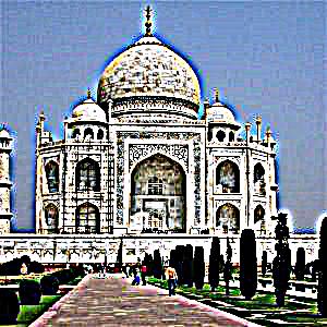


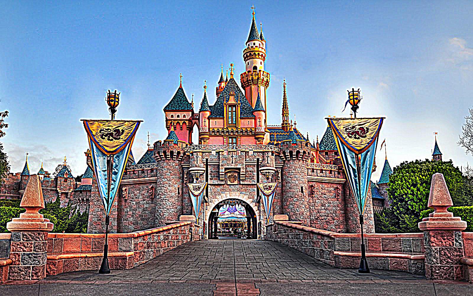
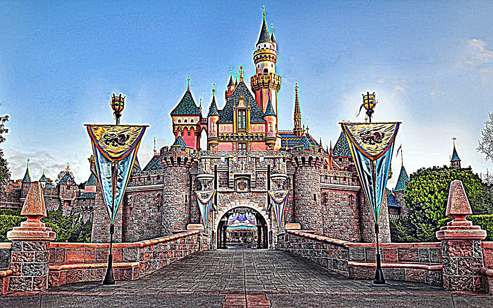


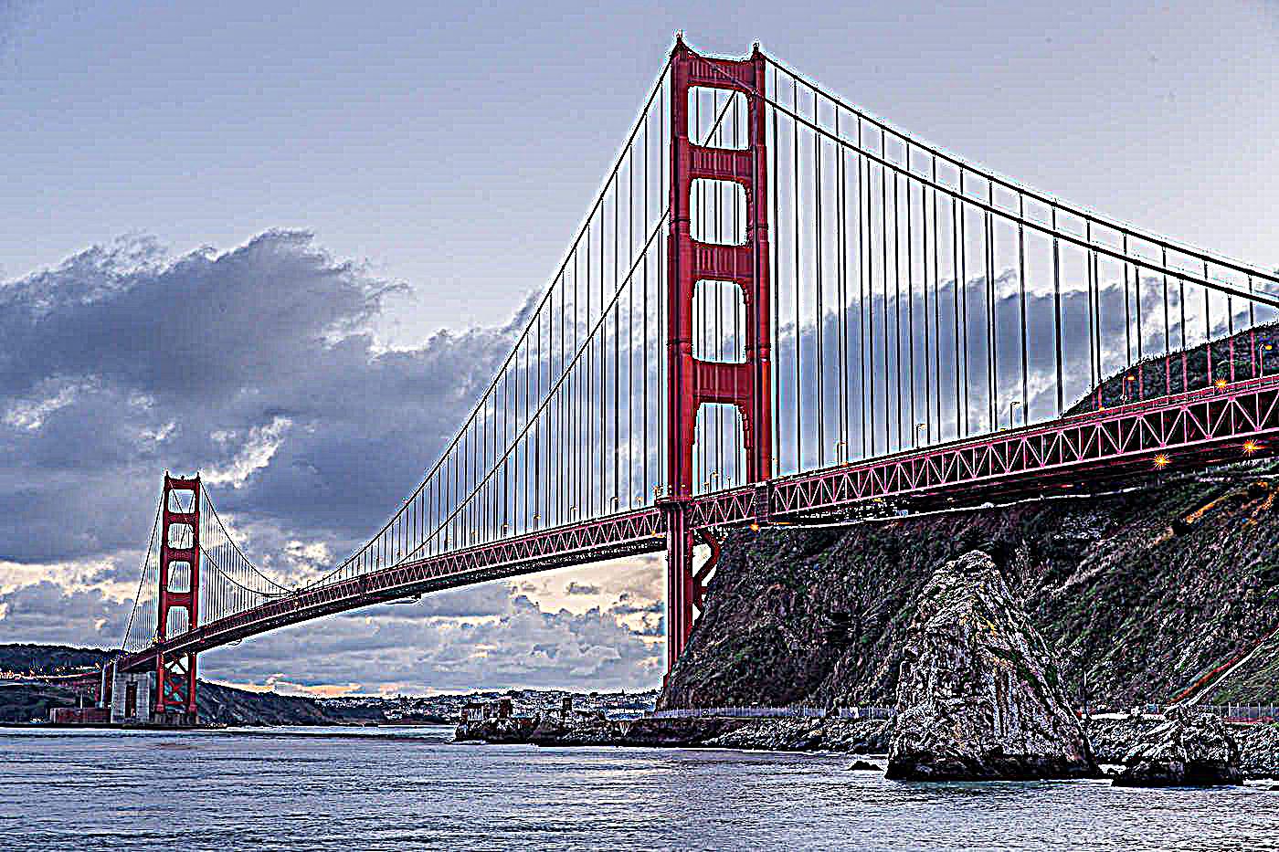
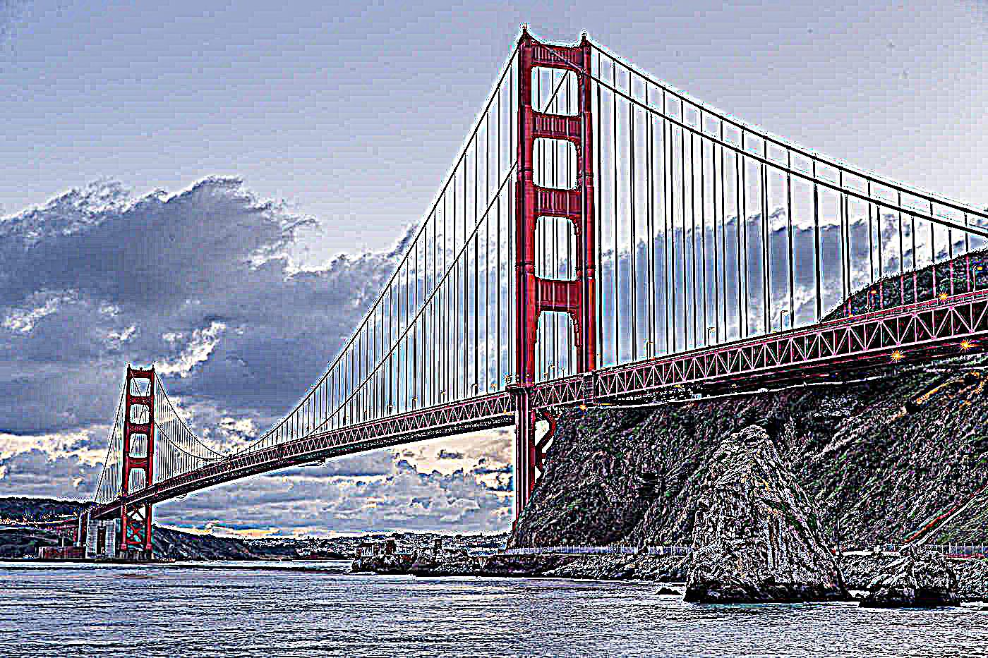
Comparing the original images to the sharpened ones, it is apparent that in general, sharpening the image with an alpha less than or equal to 1 may result in more visually appealing results but certainly a sharper looking image. After all, we are increasing the amount of high frequencies in the image so the edges of objects and structures in the image should become more pronounced and could be perceived by us as clearer. However, sharpening with an alpha of greater than 1 starts to display artifacts in the image which is exacerbated with the sharpened images using alpha = 10. The image looks over sharpened and visual artifacts are very much visible. The images no longer look real but more like an artist rendition of a real-world place on canvas.
In this section, we once again use frequencies in images in order to generate a hybrid image from two distinct images. A hybrid image is an image that we perceive differently when looked at from far away than when looked at from a close distance. From far away, we cannot distinguish the high frequencies in an image, so the image we perceive is in fact the low-pass filtered image, but when we get closer, we are able to distinguish the higher frequencies in the image so the high-frequency (or high-pass filtered) image becomes visible and overpowers the low-pass filter resulting in two different images being visible depending on how far away the viewer is standing from the image.
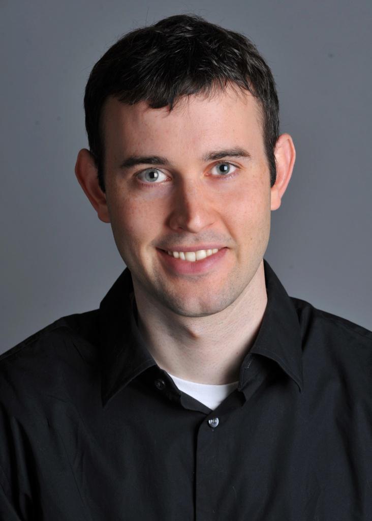
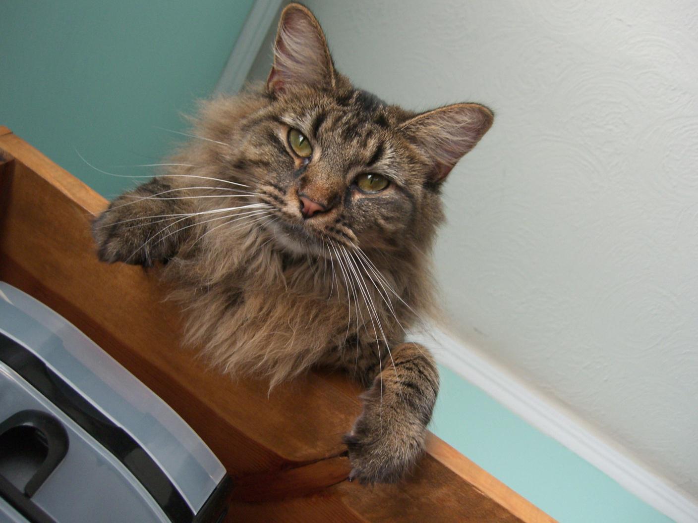
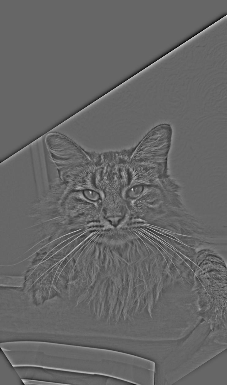
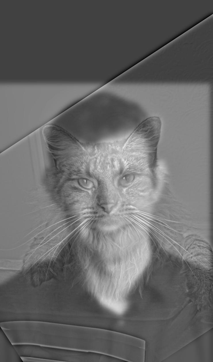
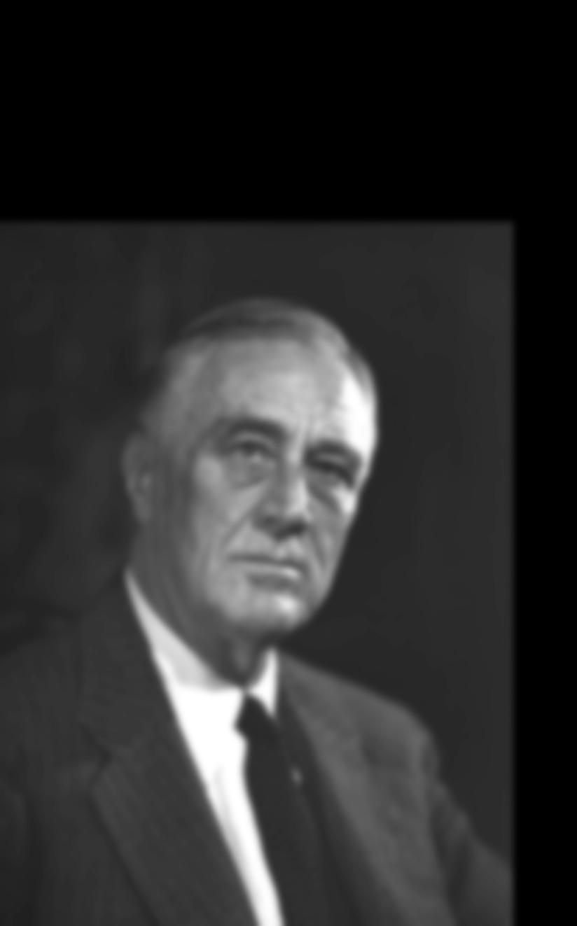
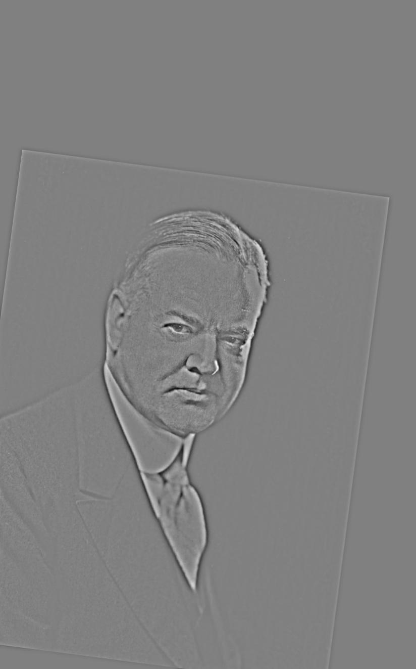
In order to generate the hybrid images, we first select to candidate images that would be good for merging. First, we run an alignment algorithm in order to match the two images and make the hybrid image more convincing. The alignment algorithm was provided with the project files and alignment was performed by selecting the eyes of the individuals in the images as the anchor points on which alignment was performed. The aligned images were then converted to grayscale in order to perform the filtering process. One image had a low-pass filter applied to it (a gaussian blur) while the other image had a high-pass filter applied to it (a Laplacian filter). The Laplacian filter was generated by creating a unit impulse of the same dimensions as the gaussian blur kernel and then subtracting the gaussian kernel from the unit impulse. This allows for the high-pass filtered image to be computed with a single convolution. Once the first image is low-pass filtered and the second image is high-pass filtered, we simply add the pixel values of the two images together.
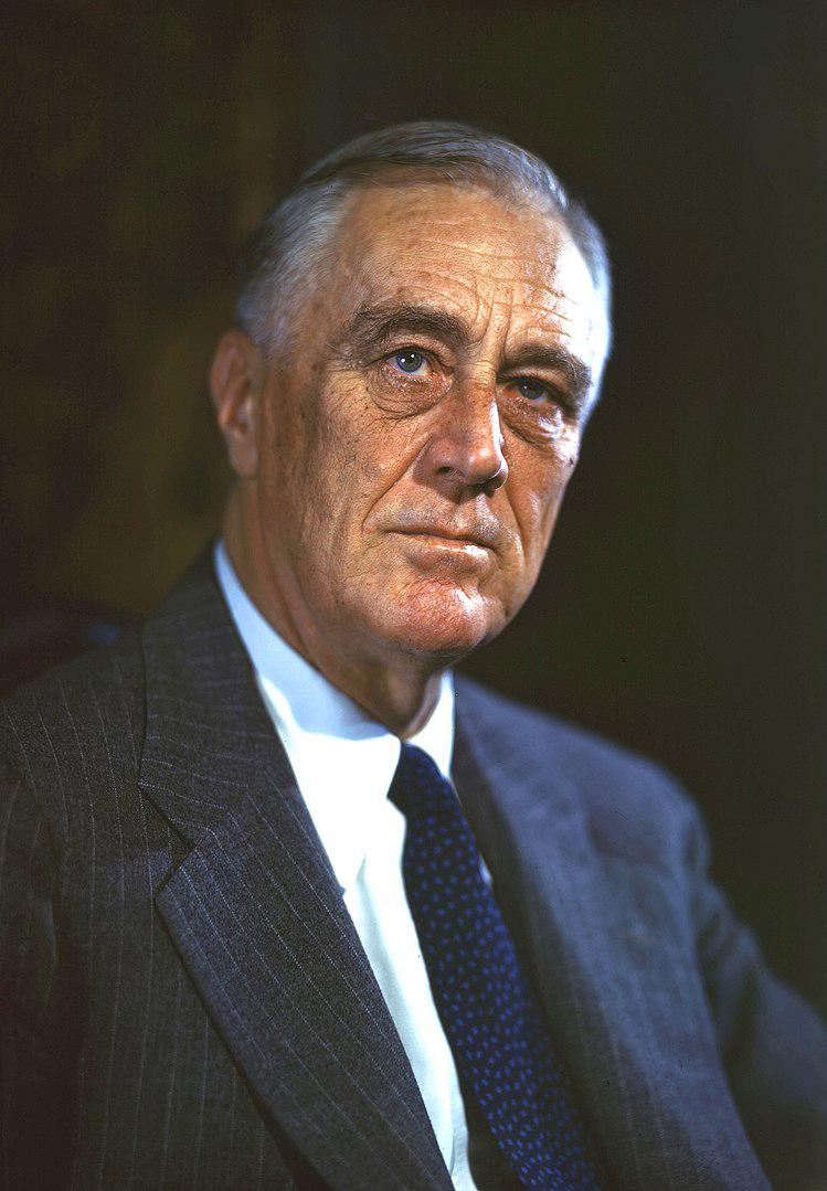
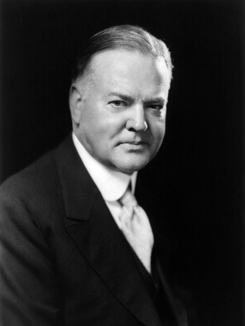
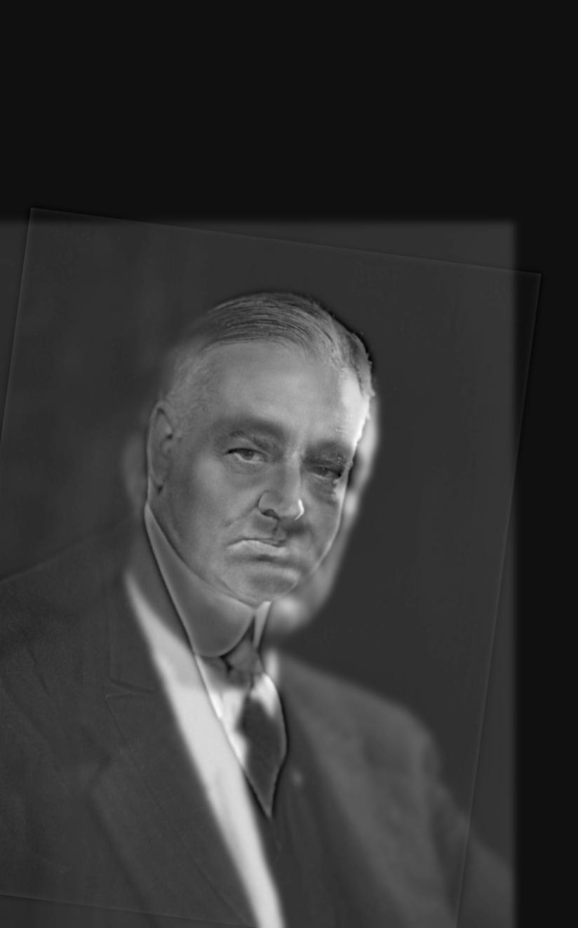
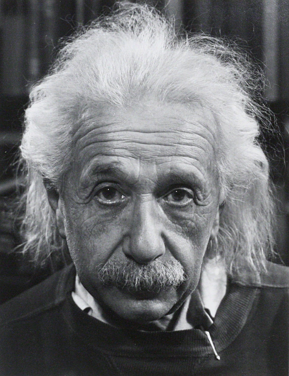
The images below show the two original images used in making each hybrid image, the associated aligned and filtered images, and the final hybrid image result. The first pairing, DerekPicture.jpg and nutmeg.jpg, were provided with the project code and were filtered using a gaussian blur with kernel width 89 and sigma 8. The second pairing, FDR.jpg and Hoover.jpg, can be found on FDR source and Hoover source. These input images were filtered using a gaussian blur with kernel width 31 and sigma 5. The third pairing, einstein.jpg and lincoln.jpg can be found on Einstein source and Lincoln source. These input images were filtered using a gaussian blur with kernel width 25 and sigma 4.

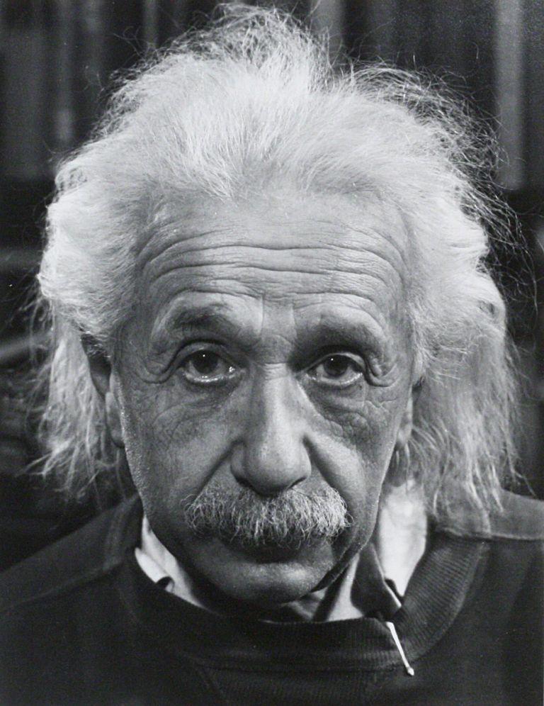
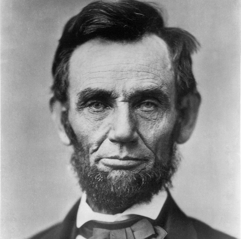
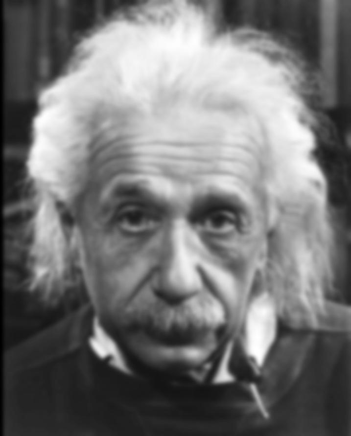
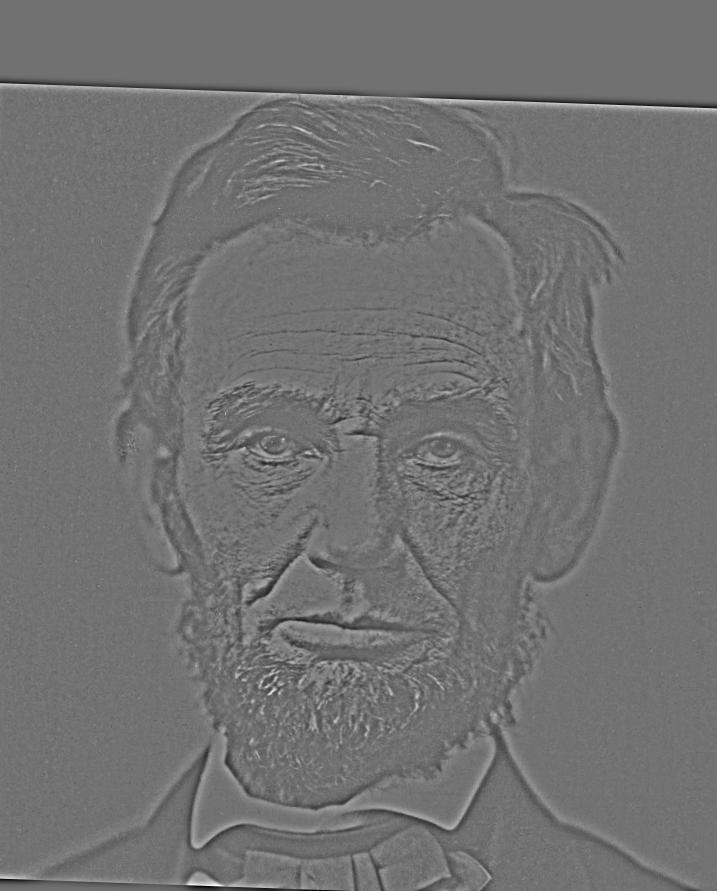
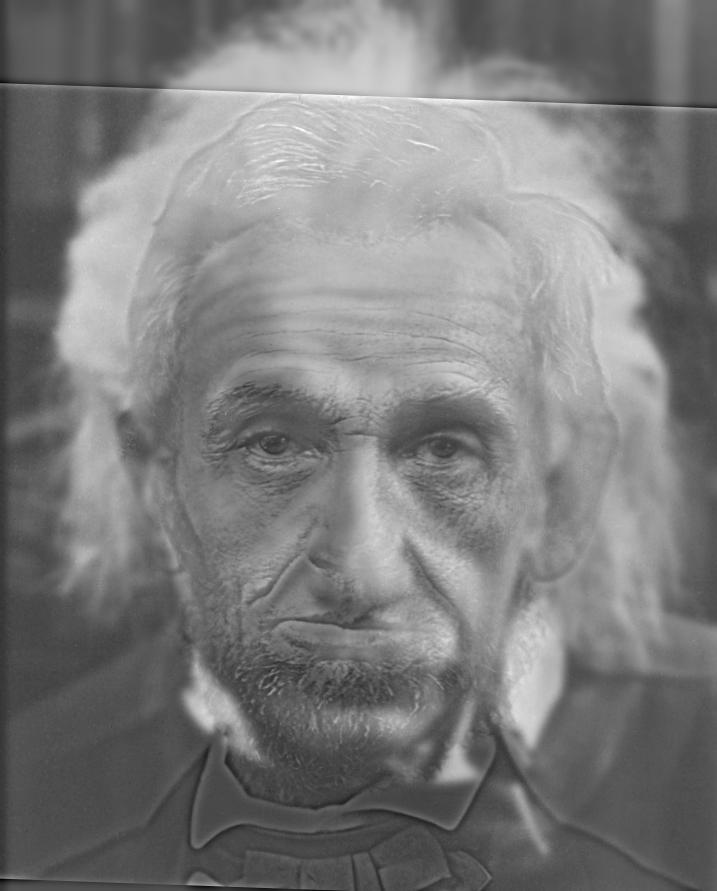
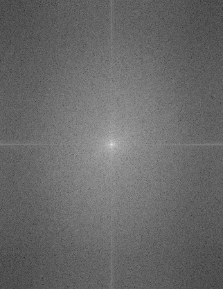
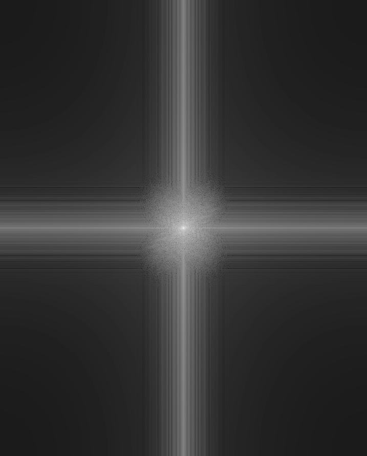
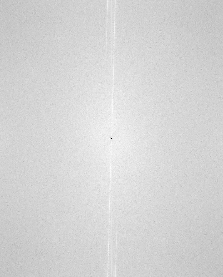
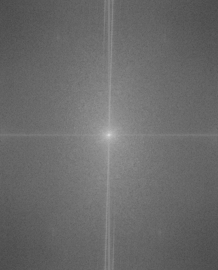
We can also visualize the process of generating a hybrid image through frequency analysis using the Fourier Transform. These images, produced in frequency space, illustrate the frequencies present in a given image with points further away from the origin, or the center of the image, being higher frequencies in the image and points closer to the origin being lower frequencies in the image. Thus, we would expect a low-pass filter to reduce the brightness in the frequency images in areas further away from the origin while a high-pass filter would increase the brightness in the frequency images in areas further away from the origin. Since the gaussian blur is not a perfect low-pass filter in the sense of perfectly eliminating frequencies higher than its cutoff-frequency, the low-pass frequency image shows higher frequencies still exist in the image, but they are significantly attenuated. Below we can see such transformations as each filter is applied to the einstein and lincoln images (all in grayscale):

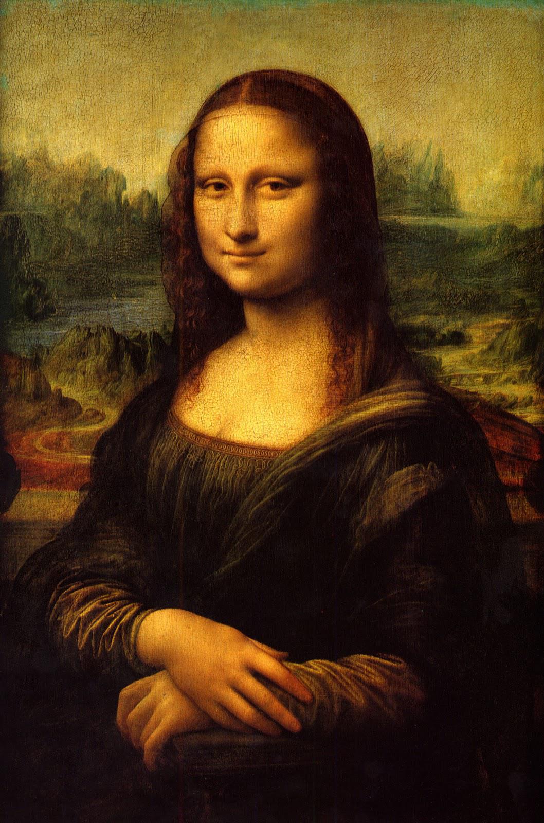
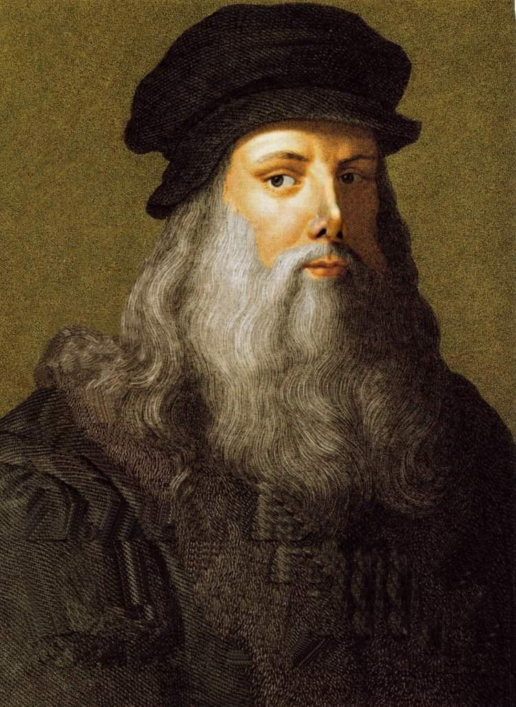
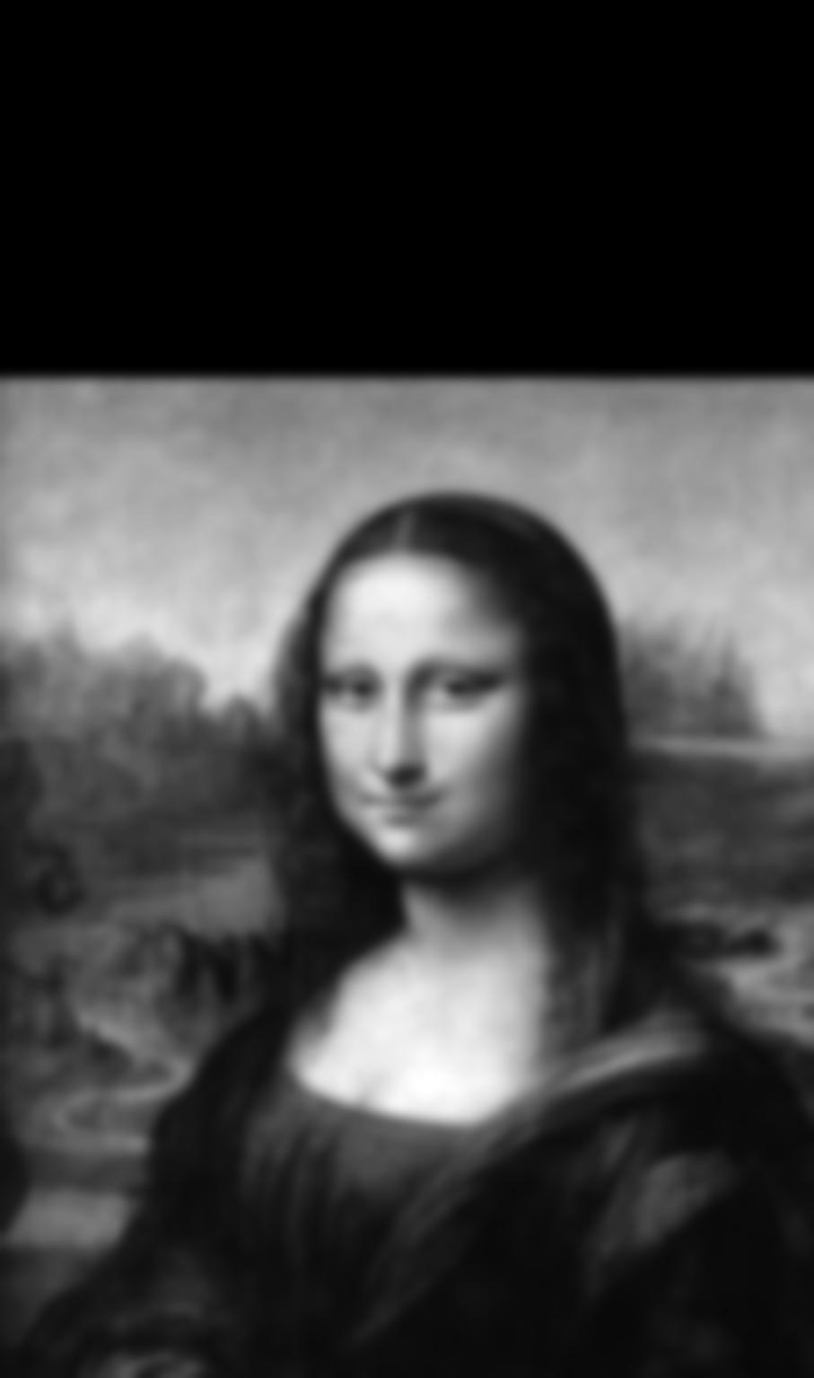
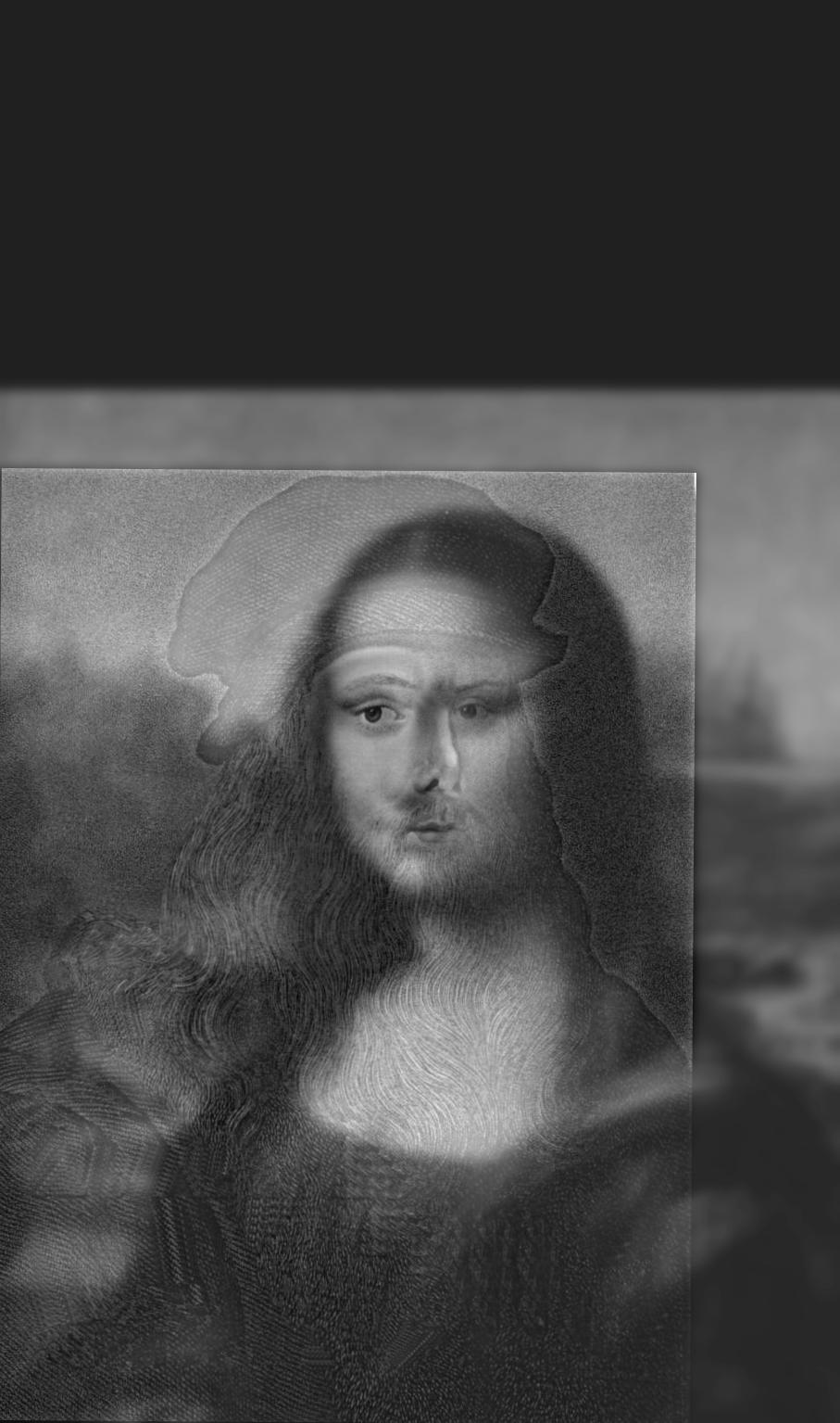
One of the hybrid images which I generated did not produce the results I was expecting. This hybrid image consisted of the Mona Lisa as the low-pass filtered image and Leonardo Da-Vinci as the high-pass filtered image. In this case, the addition of the two images to produce the final hybrid image resulted in a confusing misalignment of boundaries. Upon further inspection, I realized that even though the two images had been aligned using the eyes in both portraits as anchor points for the alignment, the portraits were facing in opposite directions; thus, the general facial features would not match up when the two images were added. This was an interesting failure case which resulted in the hybrid image being confusing to look at, neither image being easily perceived at any distance and could likely be remedied by finding portraits with generally matching facial features and directions of gaze. Below you can see the output of the hybrid image that serves as my failure case:

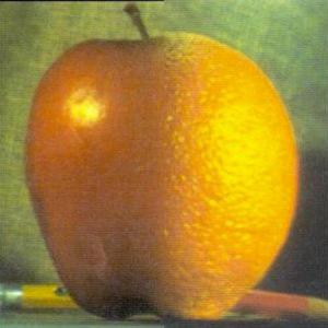
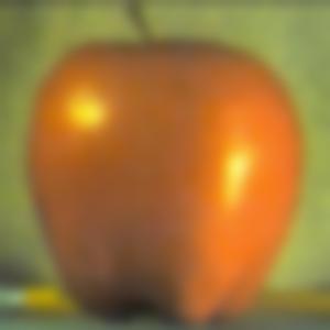
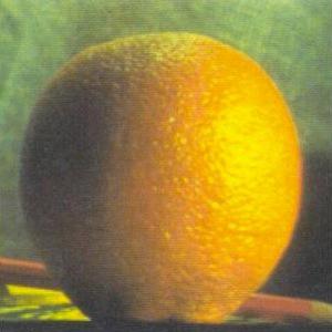
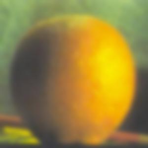
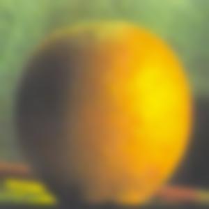
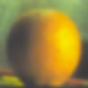
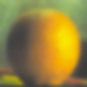
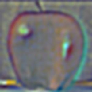
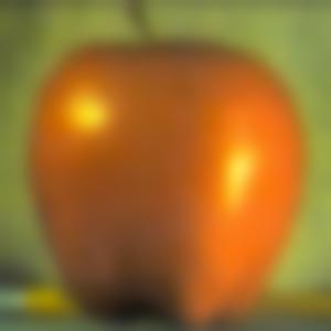
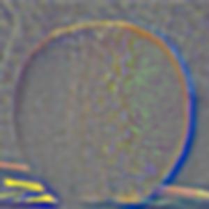
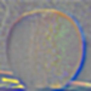
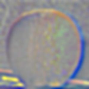
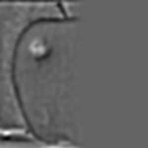
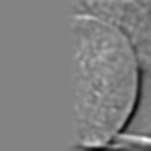
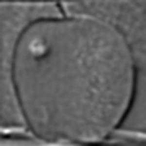
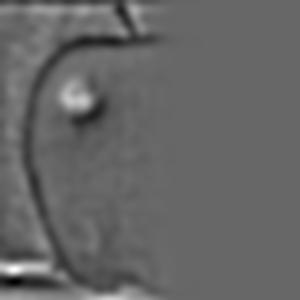
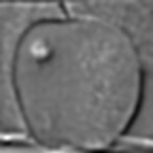
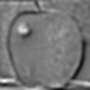
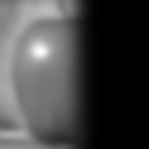
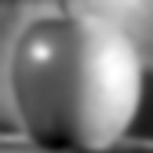
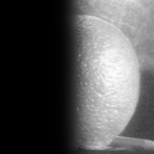
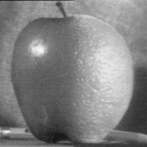
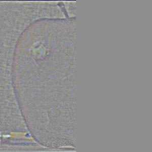
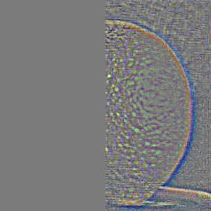
Both gaussian and Laplacian stacks are a useful means of storing multiple levels of filtered images with the same dimensions. Stacks differ from pyramids in that at each level, the image size remains the same. A gaussian stack applies a gaussian blur at each level. Thus, the original image gets more and more low-pass filtered at each level of a gaussian stack since the next level is created by applying a gaussian blur on the previous level, and so on. The parameters for the gaussian blur do not have to remain constant when creating each new level, for example the sigma can be doubled with every new level created in the gaussian stack; however, I decided to produce my gaussian stacks using the same gaussian kernel parameters with a sigma of 3 and kernel width of 18. I use 6 levels for both the gaussian and Laplacian stacks. The Laplacian stack is created from the gaussian stack in that each level is simply the difference between the corresponding gaussian stack level image and the subsequent gaussian stack level image. In essence, this difference of a low-pass filtered image with an even more low-pass filtered image creates a band-pass filtered image which we store in the Laplacian stack. The first level of the stack contains the image’s highest frequencies, the second level consists of a band of frequencies that are still high but less than the first level, the third level consists of another band of frequencies that are less than the first and second level, and so on. The last layer of the Laplacian stack is set to be the same as the last layer of the gaussian stack, since there is no next level in the gaussian stack with which to produce another band-pass filtered image; thus, the last level of the Laplacian represents all of the low frequencies which are less than all the frequency bands of the higher levels. Another convenient property of a Laplacian pyramid is that all the levels in the Laplacian stack can be summed to reproduce the original image, which is a property we use to reconstruct the final grayscale and color melded images. Below are all the levels produced for the Gaussian and Laplacian stacks when creating the grayscale version of the oraple.

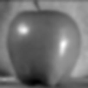

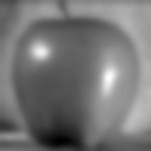
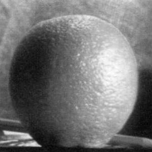


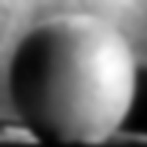
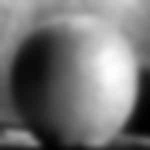
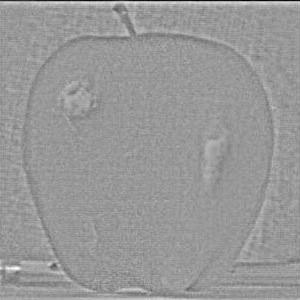
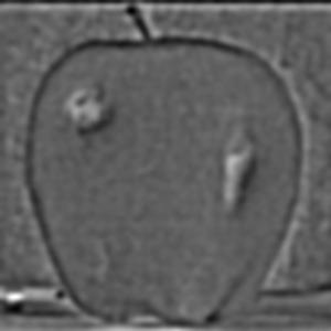
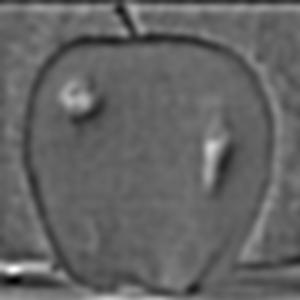


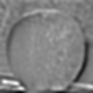

The following section will show the Gaussian and Laplacian stacks used to produce the color version of the oraple. The key difference between the grayscale and color computations is that the grayscale stacks only consist of one data channel, grayscale, whereas the color stacks have three separate data channels (red, green, and blue). Each color channel has its own gaussian and Laplacian stack which I have recombined at each level and normalized pixel values using minmax normalization. The displayed images are the recombined color versions of these three color channels for the gaussian and Laplacian stacks. In section 2.4 following this section I will display the produced melded images as well as the applied vertical alpha mask at different levels of the Laplacian stack but before doing so, below are the gaussian and Laplacian stacks used to produce the color image of oraple.


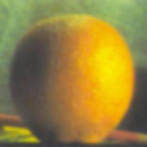
In this section, we use the generated gaussian and Laplacian stacks from the previous part in conjunction with a gaussian stack of an alpha mask in order to perform multiresolution blending. To create the alpha mask used in producing the oraple image, I created a new 2D array of equal dimensions to the two input images and assigned a value of 1 to all pixels which were to the left of the vertical midpoint line of the image frame and assigned a value of 0 to all pixels which were to the right of the vertical midpoint line of the image frame. I then created a gaussian stack consisting of the same number of levels as the input image stacks, at each level further blurring the mask to smoothen out the boundary between black and white. Additionally, after some experimentation, I settled on using a larger gaussian filter on the alpha mask when generating its gaussian stack when compared to the gaussian filter used to generate the gaussian stack of the input images. The gaussian filter used on each level of the mask’s gaussian stack had a sigma of 9. I observed that using a bigger gaussian filter on the mask removed some harsh edges on the boundary near the top and bottom of the image (see also Most Important Thing I Learned from this project section for another insight I came across through experimentation to smoothen the boundary between these two images).
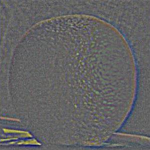
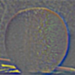
After creating the gaussian stack for the alpha mask, I then proceed to apply the mask to each respective Laplacian level for the two input images. In producing the grayscale oraple, this is done by simply multiplying each level of the input image Laplacian with the respective layer of the mask gaussian stack. One image has the mask applied as is, the other image has the mask flipped which is done by performing an element-wise subtraction of 1 minus the appropriate mask level from the gaussian stack. In producing the color oraple, the process is pretty much the same with the exception that it is performed on three separate color channels instead of just a single grayscale channel. Included below are what the Laplacian stacks for each image in grayscale look like after applying the mask. Since the Szeliski book adopts the notation that the first layer of the stack is level 0 instead of my previous notation of level 1 being the top level of the stack, the following images will be labeled levels 0 through 5 instead of 0 through 6 in the interest of modeling figure 3.42 on page 167 of the book for both the grayscale and the color outputs.

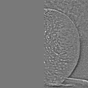
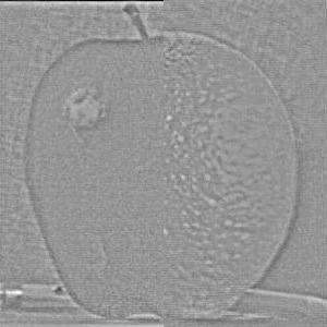

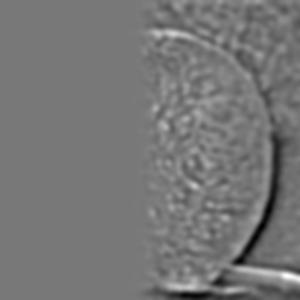
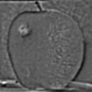

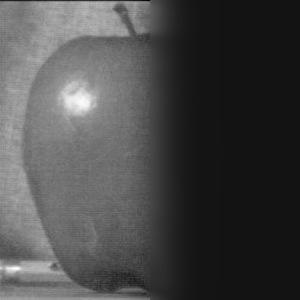
And included below are what the Laplacian stacks for each image look like in color after applying the mask.
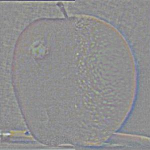
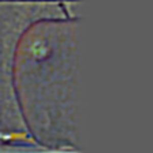
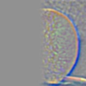

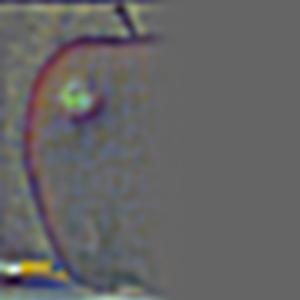
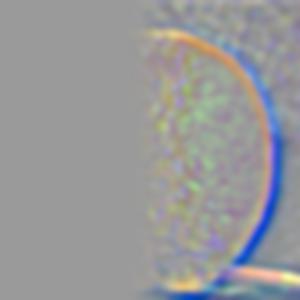
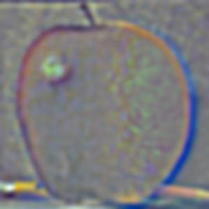
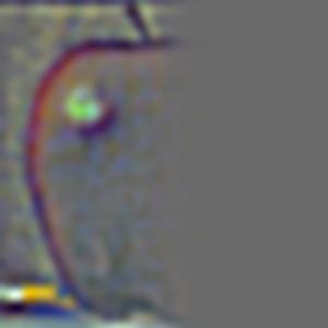
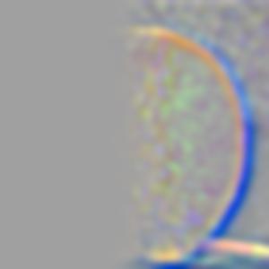
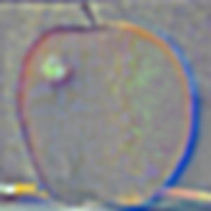
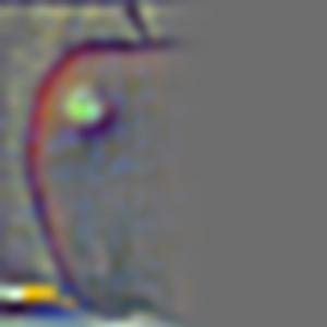
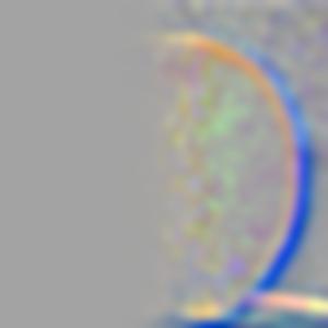
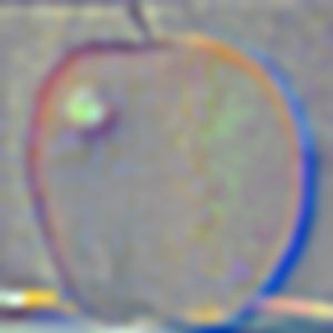


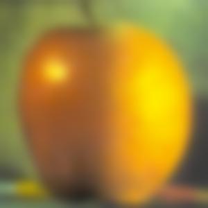
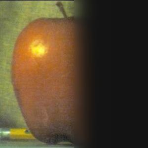
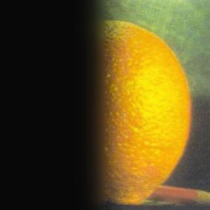
Although the end results are visisble above, the fomalize the process I reitterate the steps required to produce the final merged image. Now both images have a mask applied to them on all levels of their Laplacian stack, in this case only the left half of the apple is visible and the right half of the orange is visible. To reconstruct the two individual images, we just stack their respective Laplacian stacks by summing all the levels. Doing so in grayscale produces the following two images:
And doing so in color produces the following two images (the Laplacian stacks for the red, green, and blue channels are first summed together and then the color image is created from the three summed color channels):
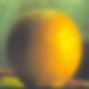
All that is left now is the sum the two above images together in order to produce the final melded image which is displayed below in both grayscale and color.
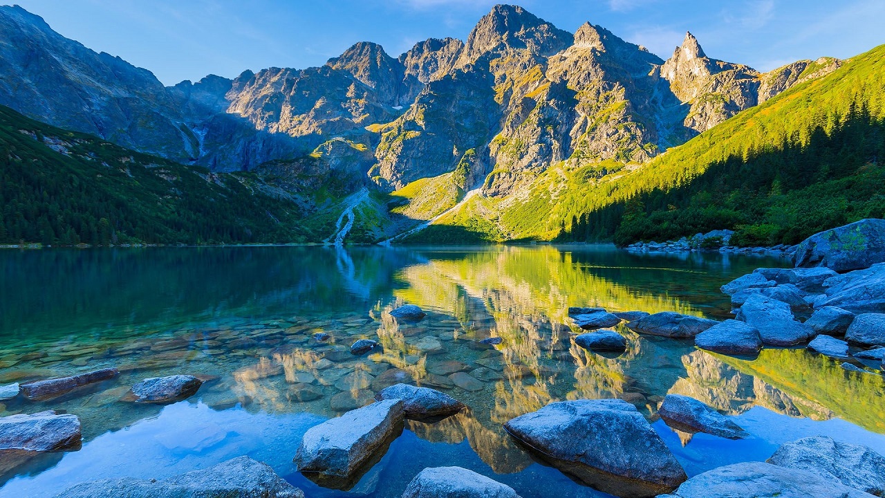
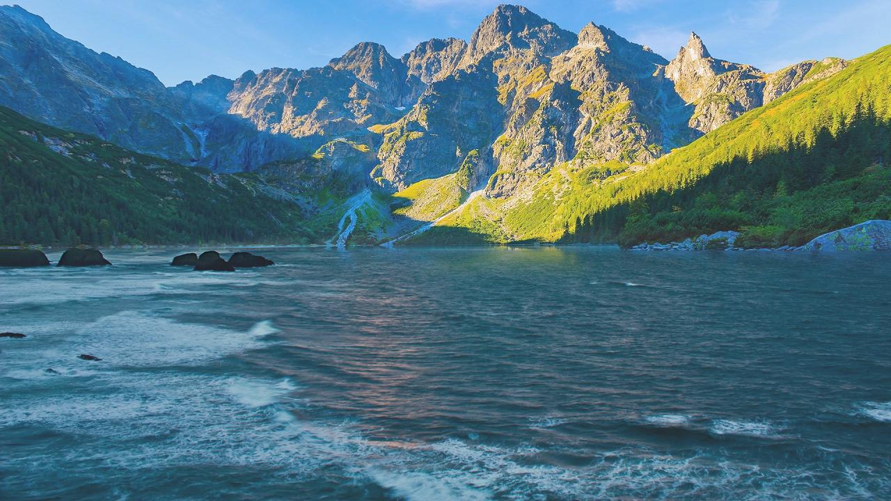
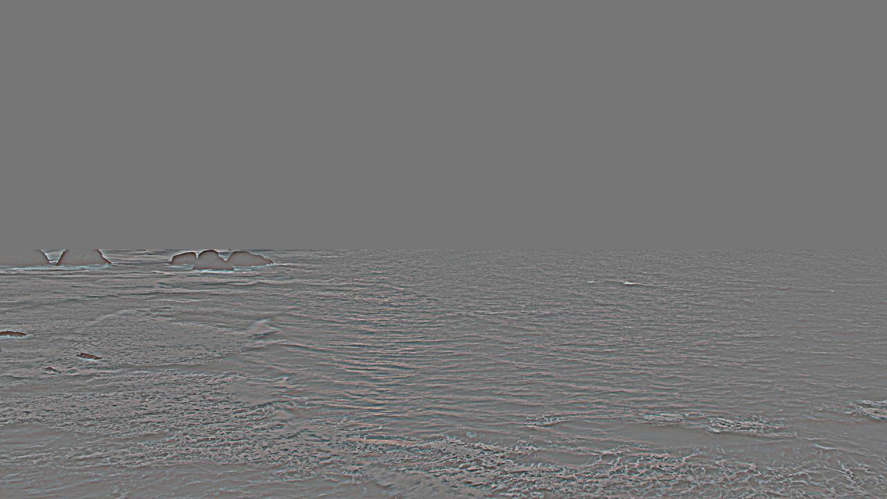
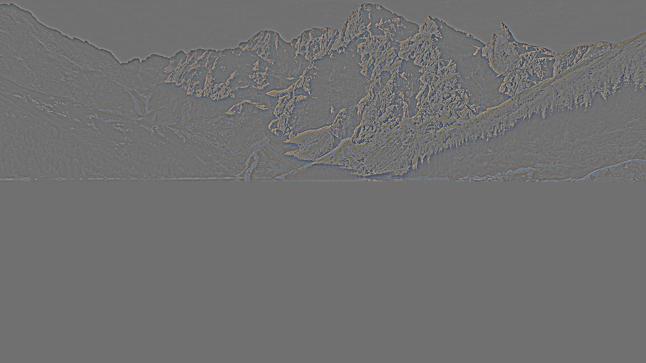
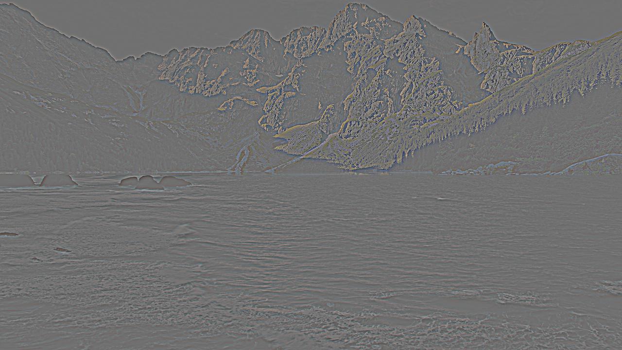
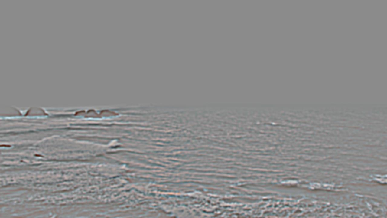
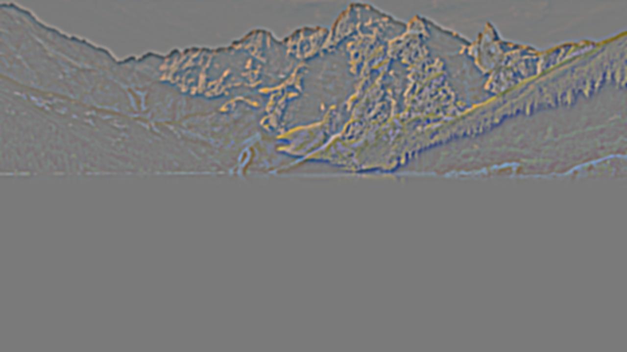
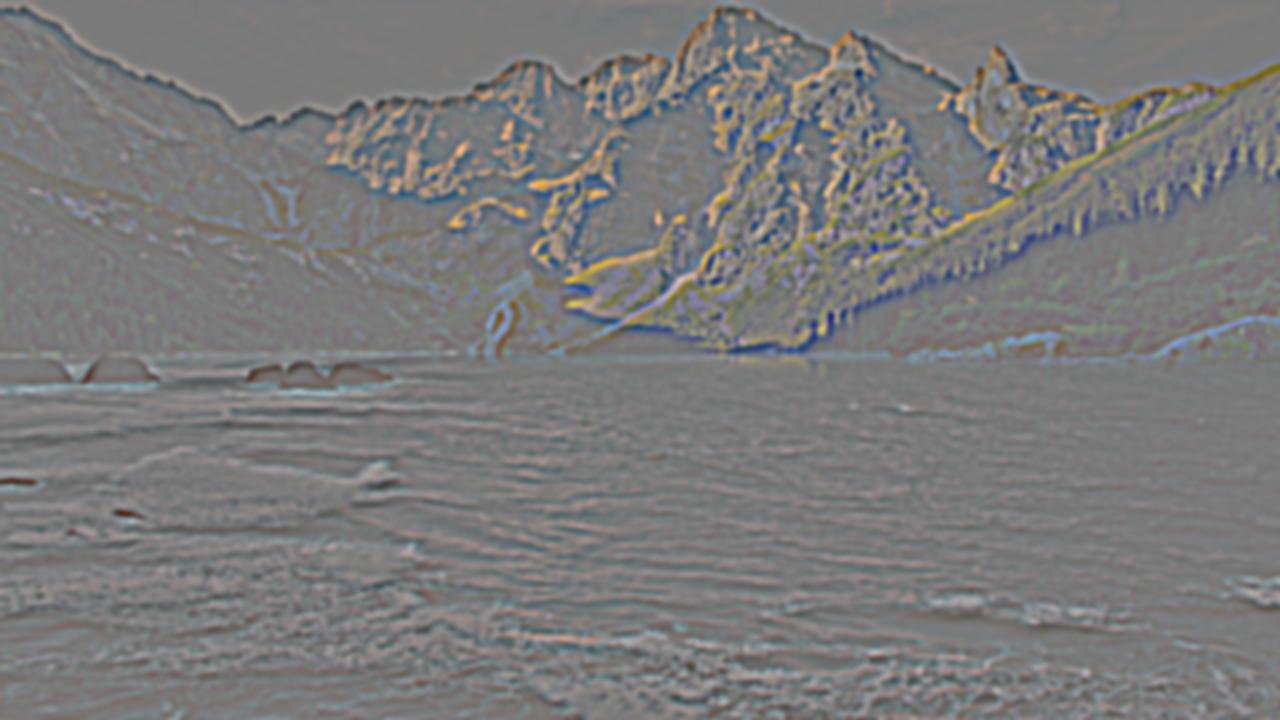
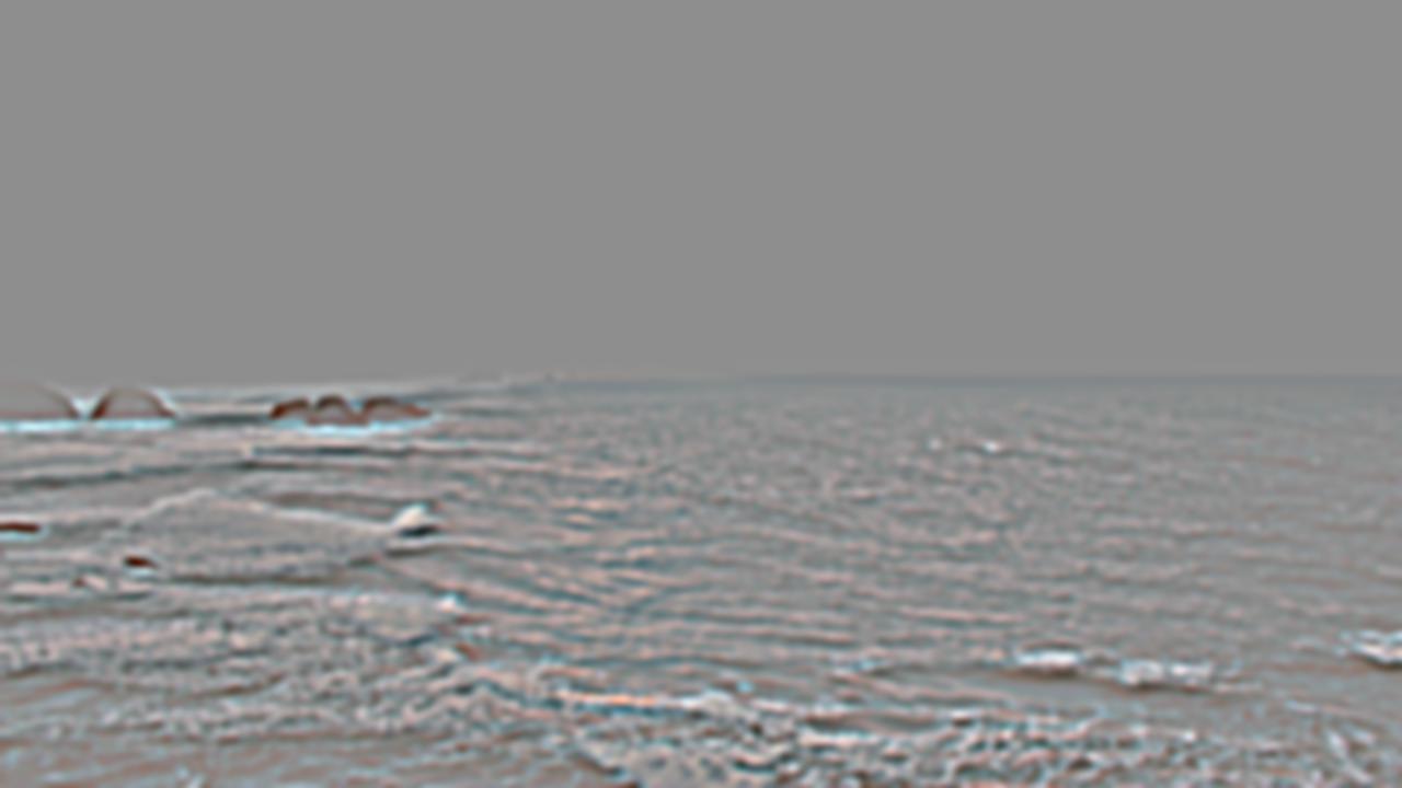
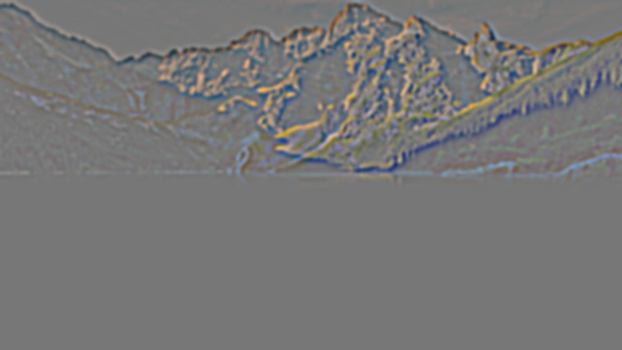
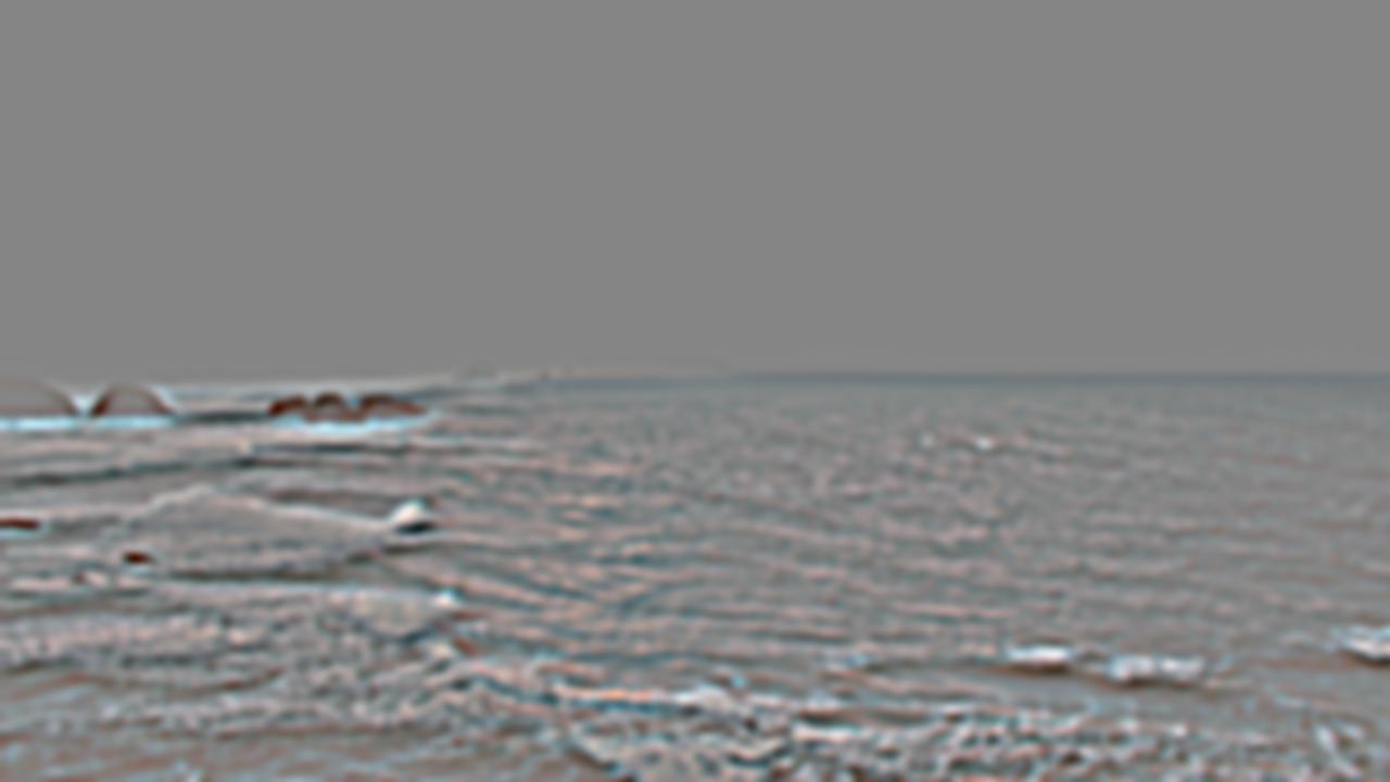
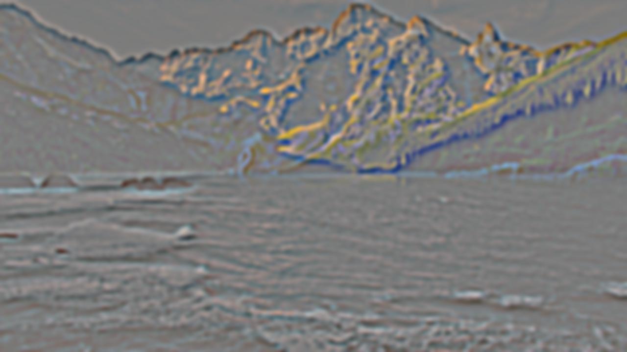
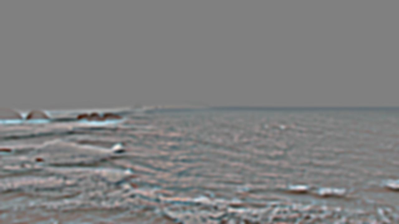
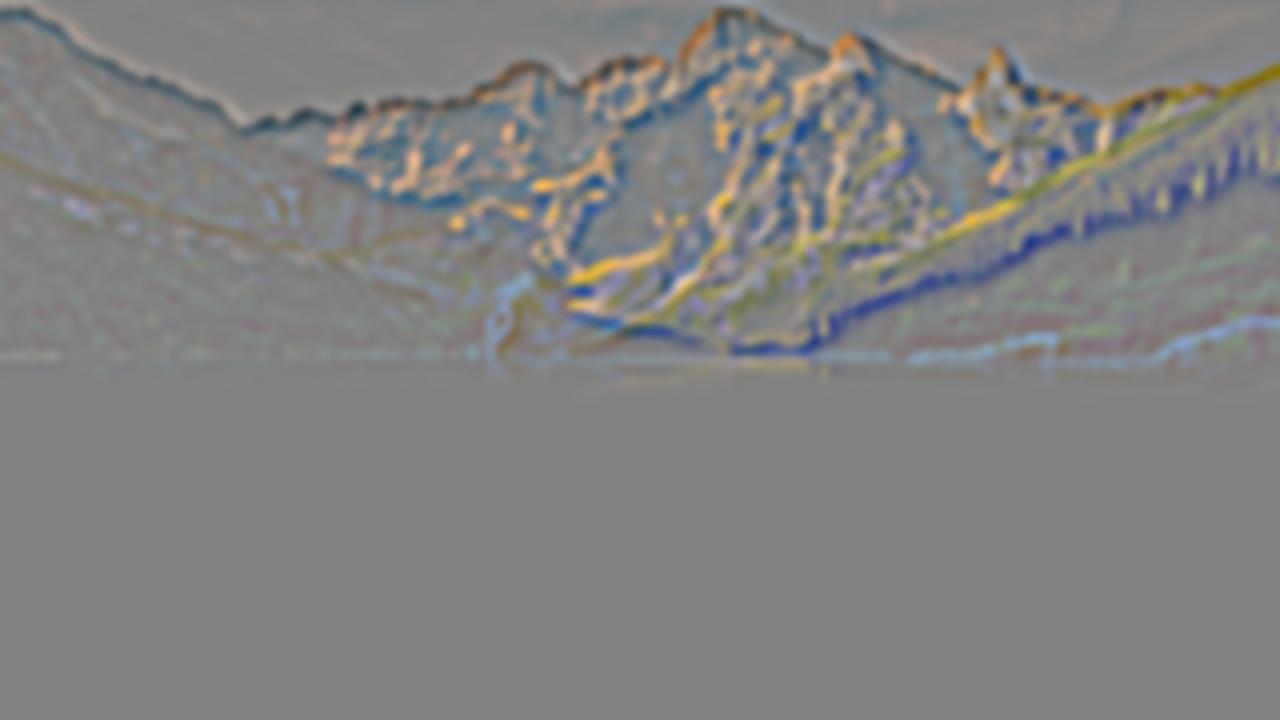
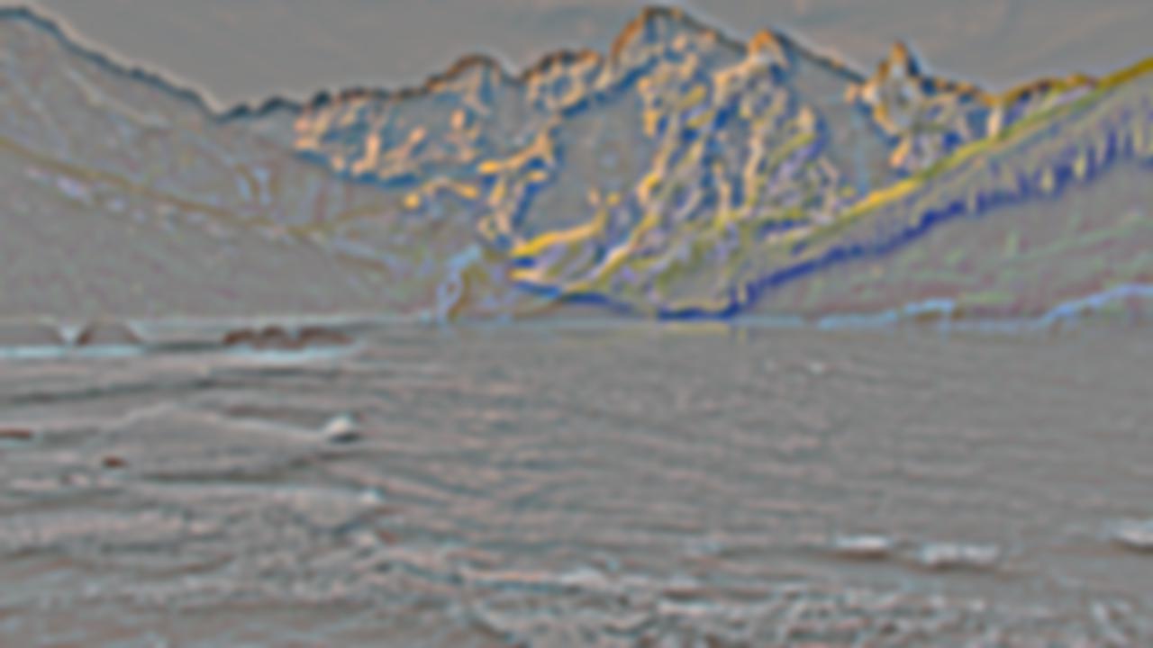
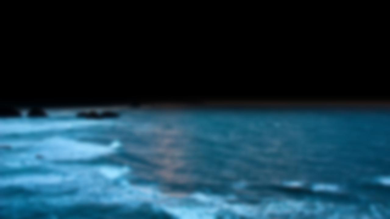
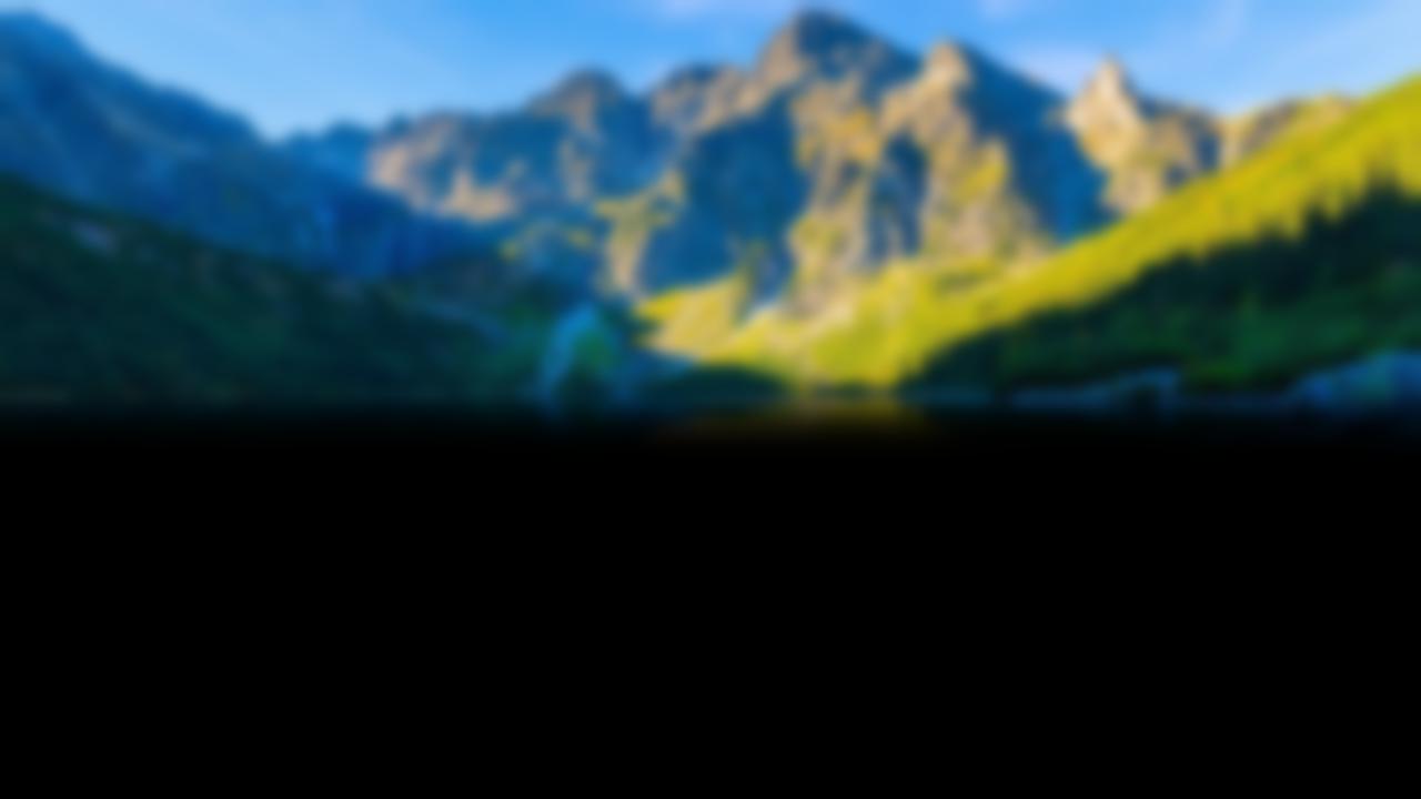
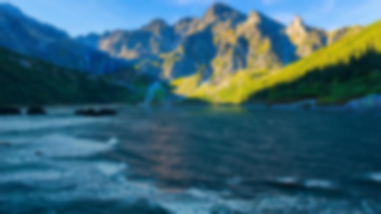
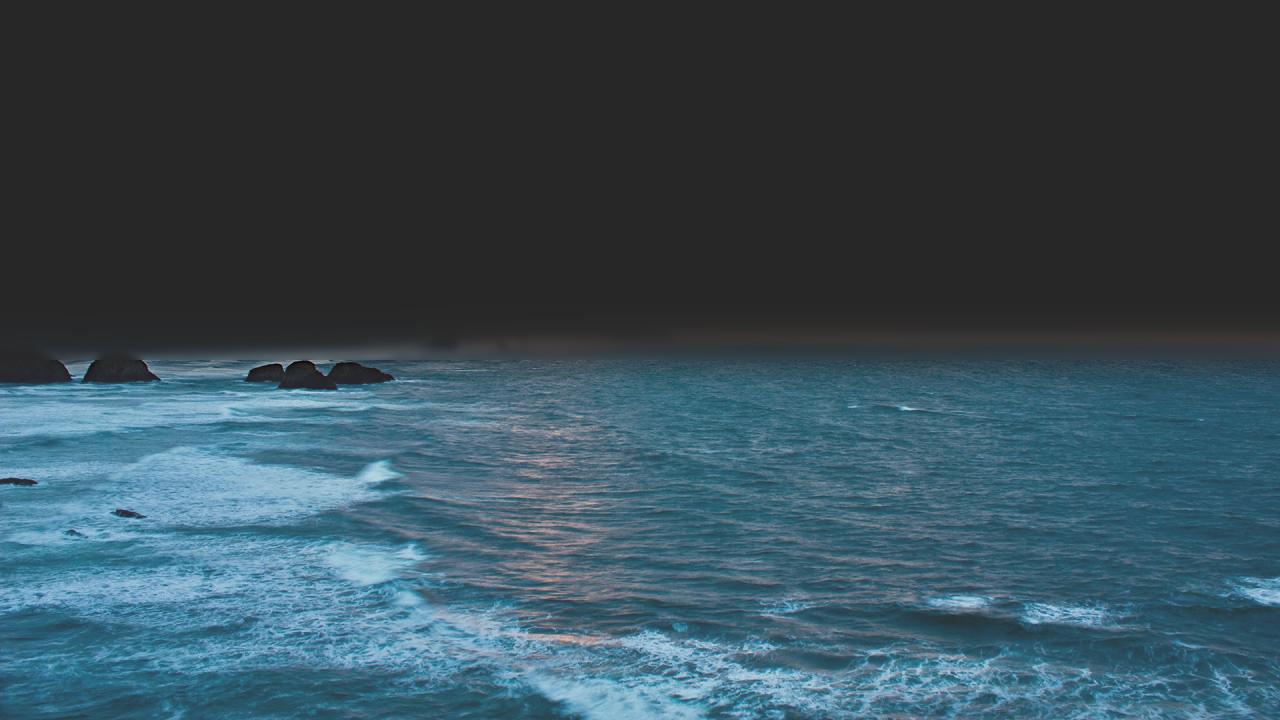
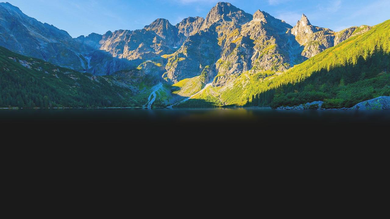
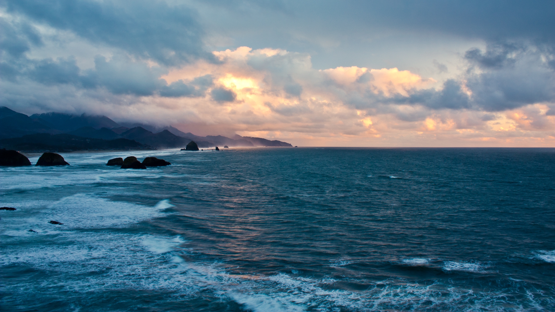
One additional example of multiresolution blending which I performed was between ocean.jpg and mountain.jpg which can be found at ocean source and mountain source. For this blending procedure, I defined a horizontal mask that would match up closely with the horizon from the ocean picture, which was relatively the same height as the where the water ended in the mountains picture. I utilized the algorithms we learned in this assignment to attempt to modify the calm lake in the mountains picture to display the turbulent waters from the ocean picture. The end results came out surprisingly well. Below are the two input images along with the final color blended image.

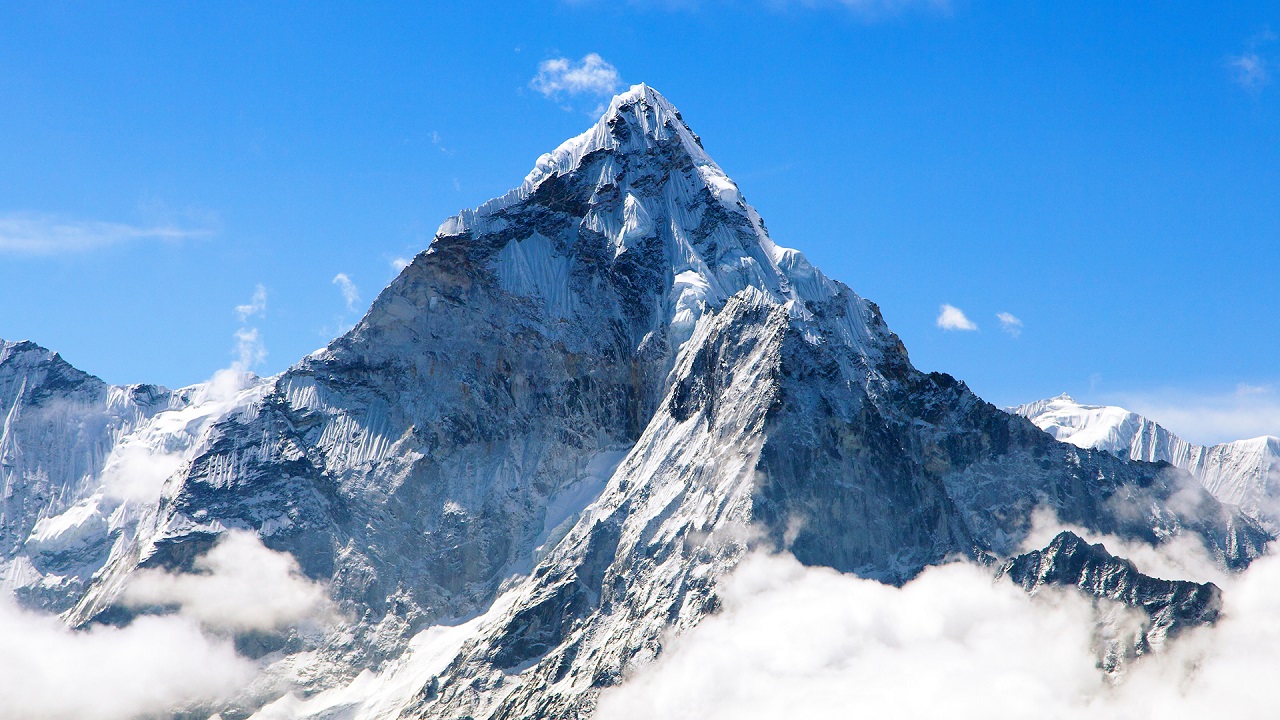
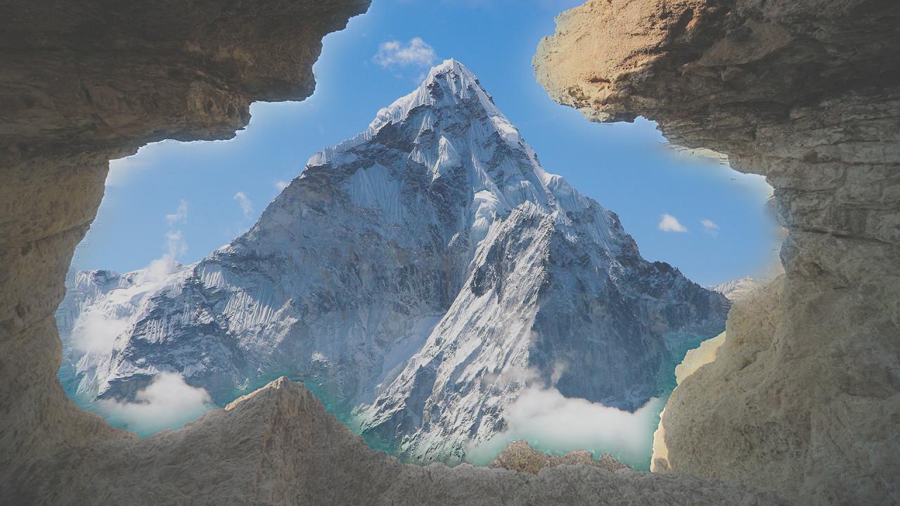
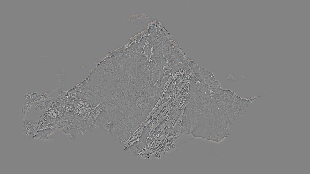
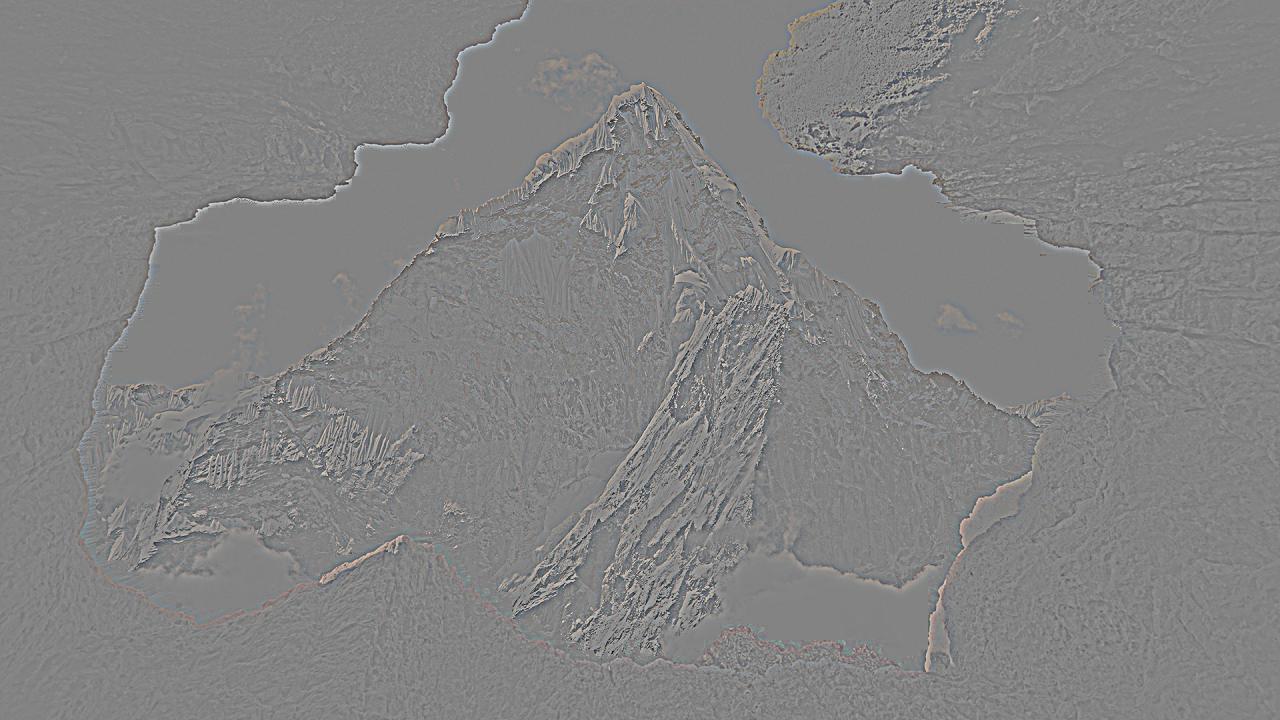
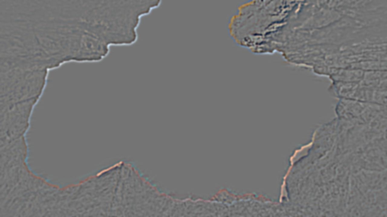
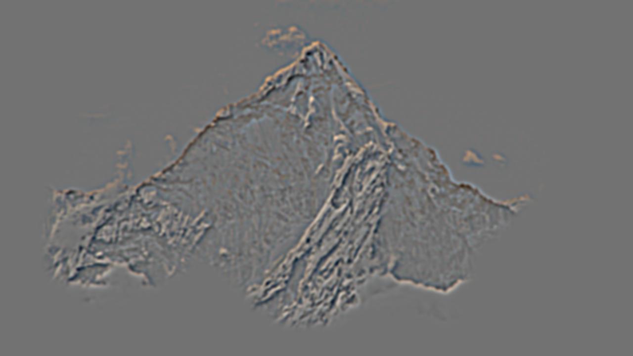
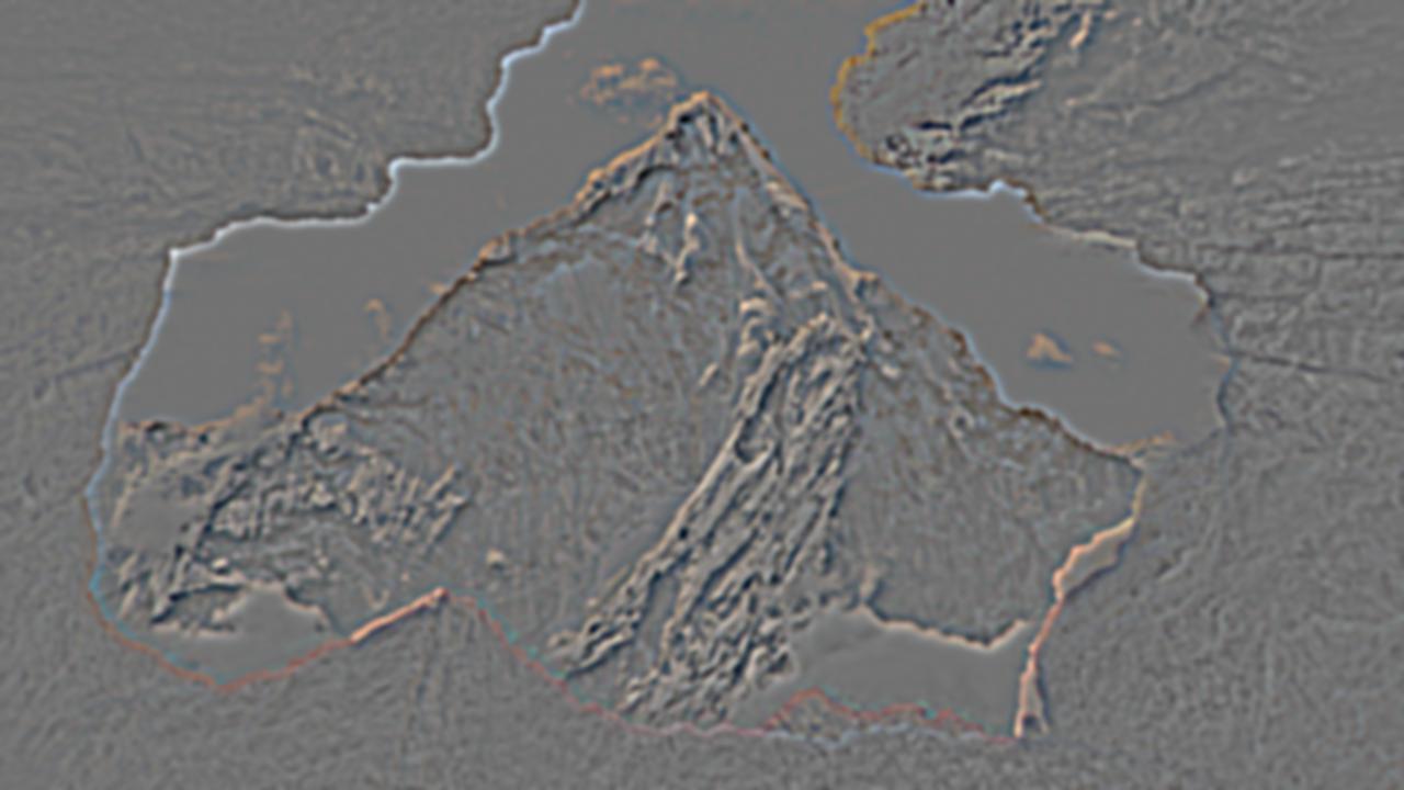
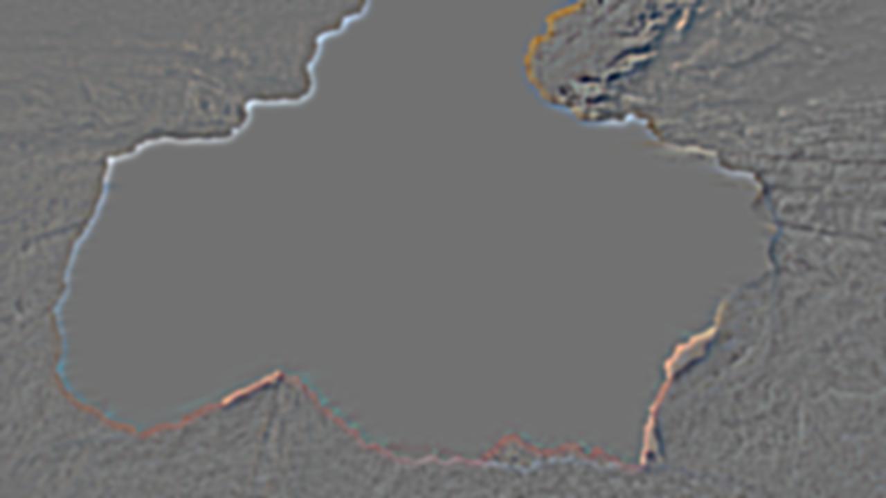
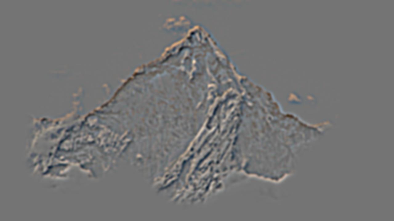
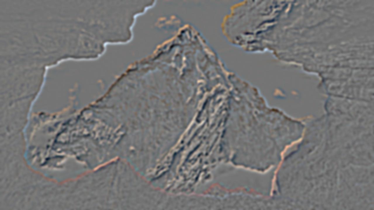
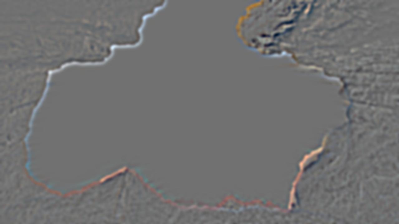
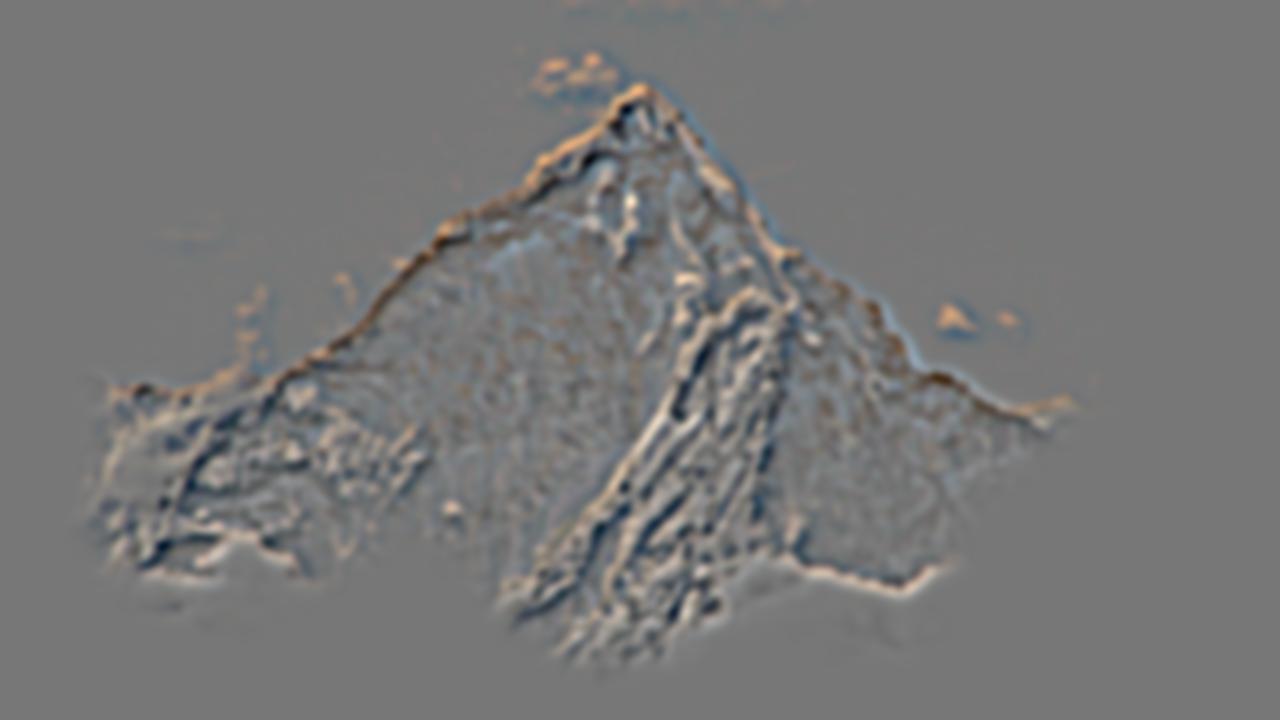
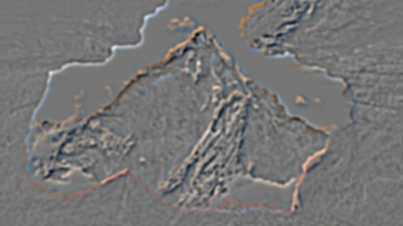
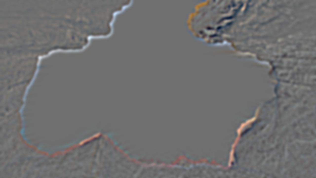
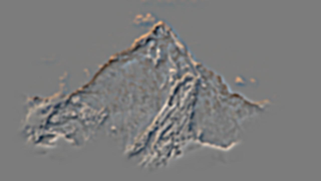
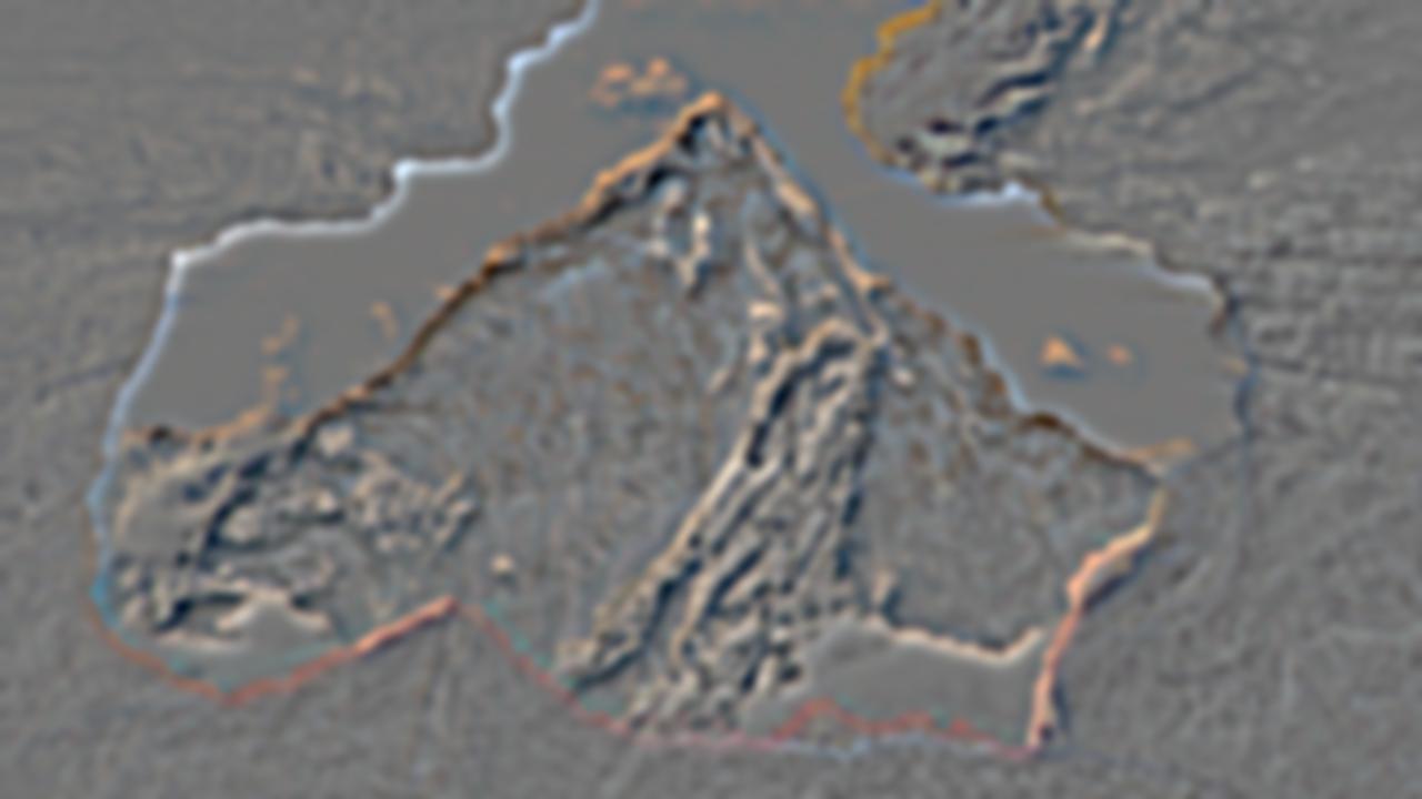
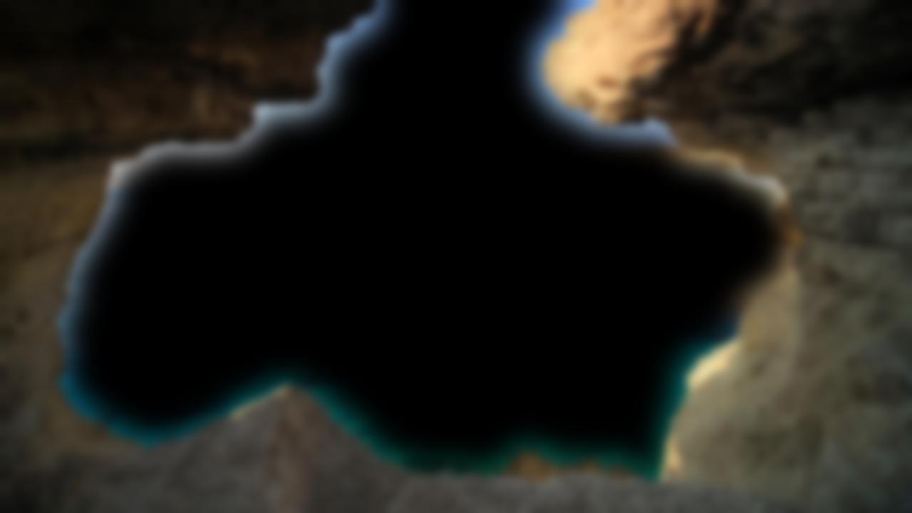
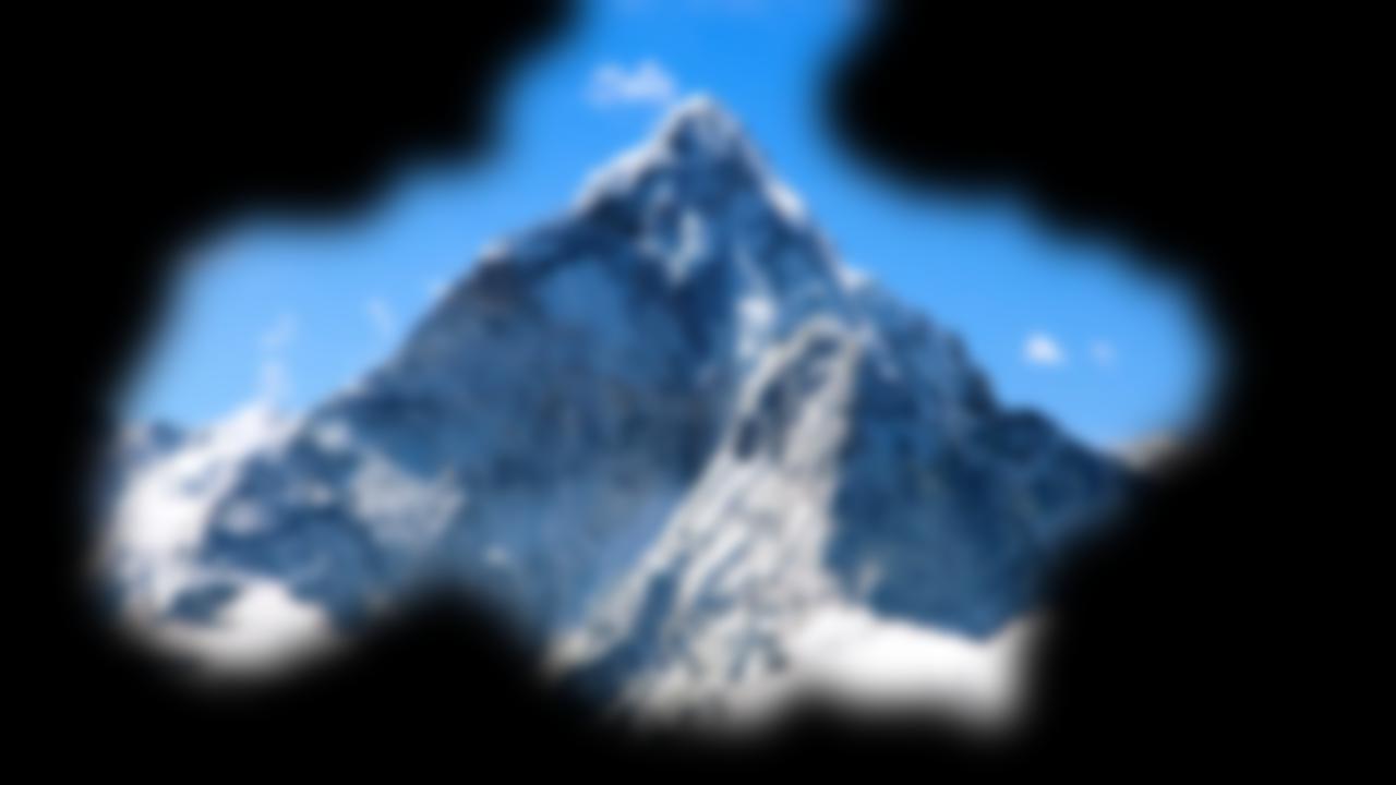
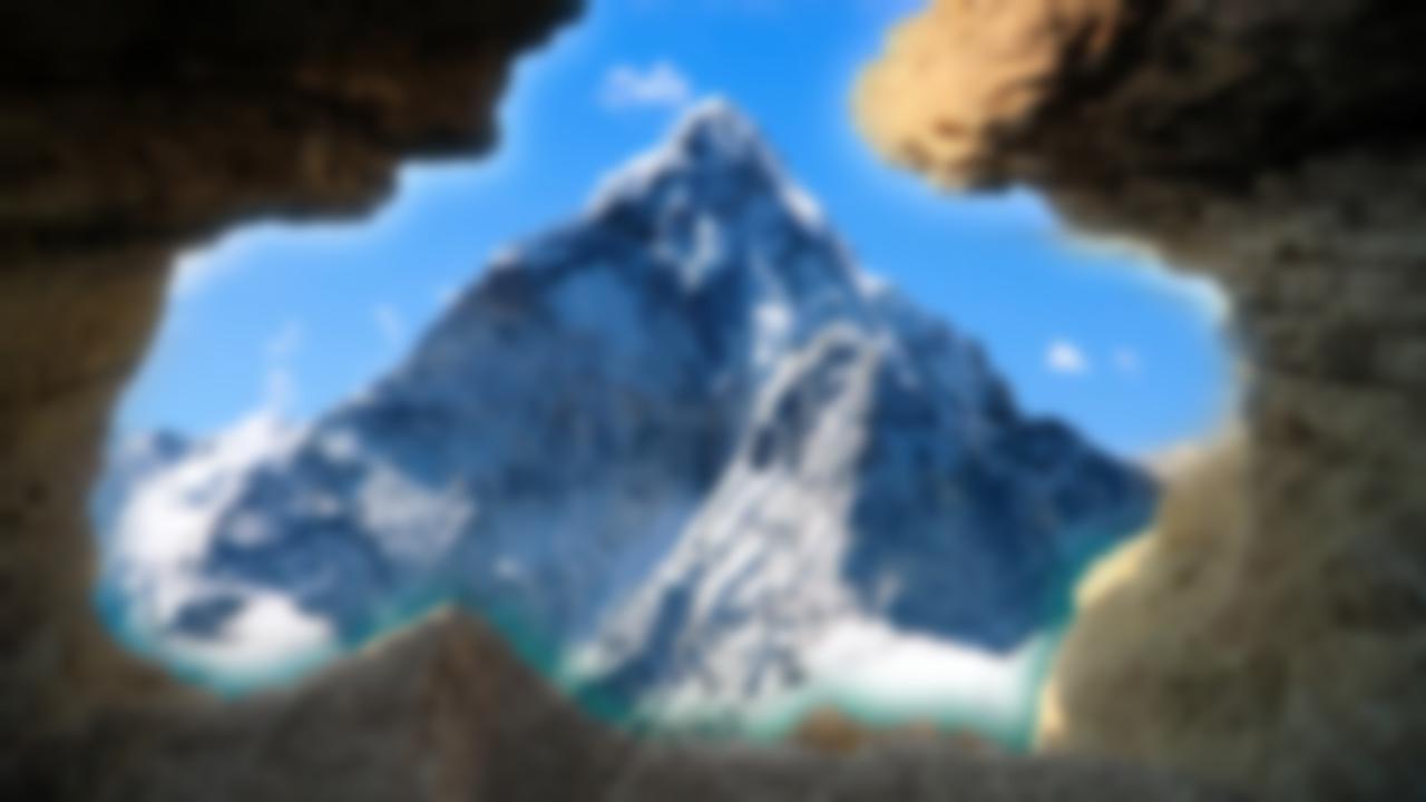
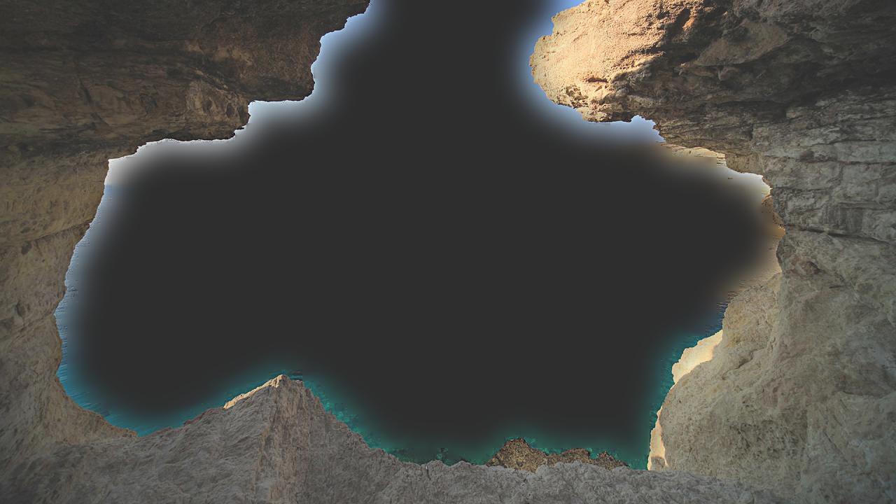
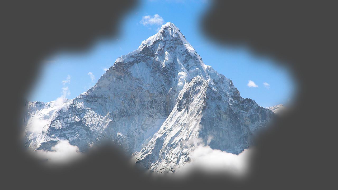
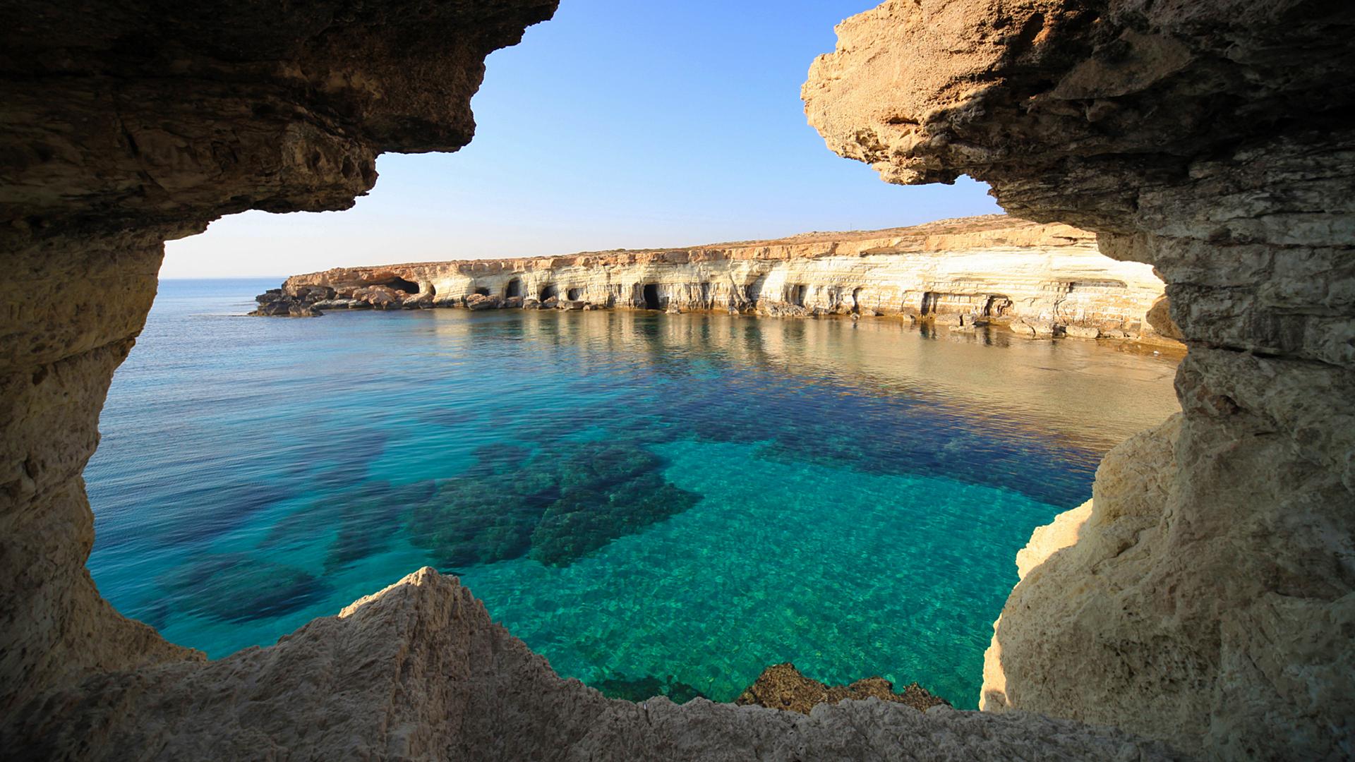
I also created a second additional multiresolution blending example between viewport.jpg and everest.jpg which can be found at viewport source and everest source. For this blending procedure, I defined a much more complex mask that would outline the viewport hole of the sea rocks. I created a rough sketch of the mask using Paint on Windows and processed the mask in-code to create the binary pixel values of 1 and 0 we need for the mask. The blending process was the same from this point forward. The blended output image looks good though a bit hazy around some of the sea rocks which is not the fault of the algorithm but instead of the mask not being draw very precisely. Overall, the output image still looks very good and the two input images along with the final color blended image are displayed below.

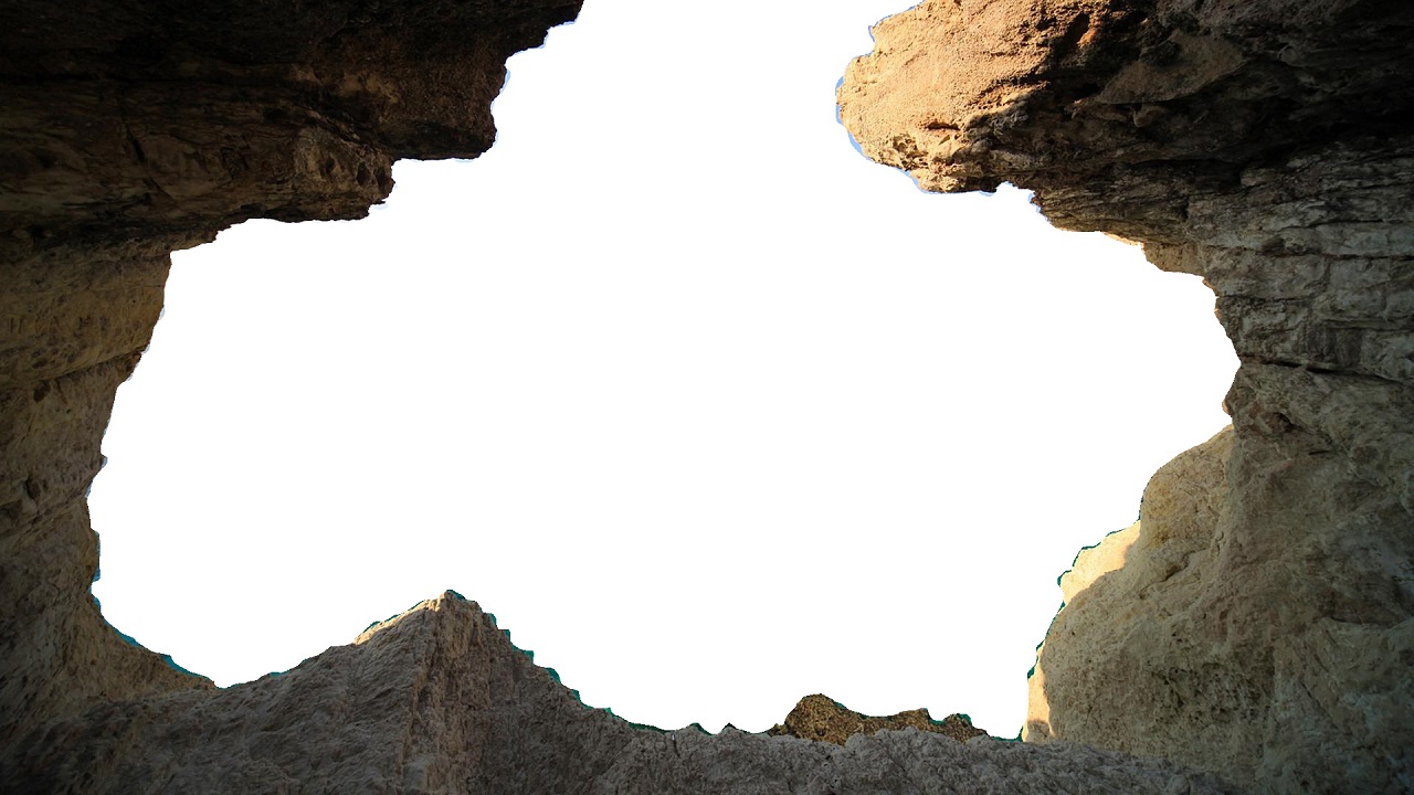
And below is the mask used to produce the blended image between viewport.jpg and everest.jpg:
From experimentation, one thing that I learned from this section was that by applying a larger gaussian blur on the gaussian stack, and then creating the Laplacian stack from the gaussian stack, the blending of the two images was not as smooth. Upon inspecting the Laplacian stack, I realized that applying a much larger gaussian blur resulted in most of the high-frequency features being present on the first level of the Laplacian stack, which had a non-blurred mask applied to it. Consequently, most of the image information was stored in the first level of the Laplacian stack which had a very abrupt blending edge which was visible in the final image. In order to create a smother transition between the two images, I reducing the blurring on each level of the gaussian stack which in turn resulted in less high frequencies stored in the first level of the Laplacian stack and more frequencies distributed over the lower levels of the stack which received a more blurred mask. Thus, the final image had a more seamless transition between the two images rather than an abrupt one.
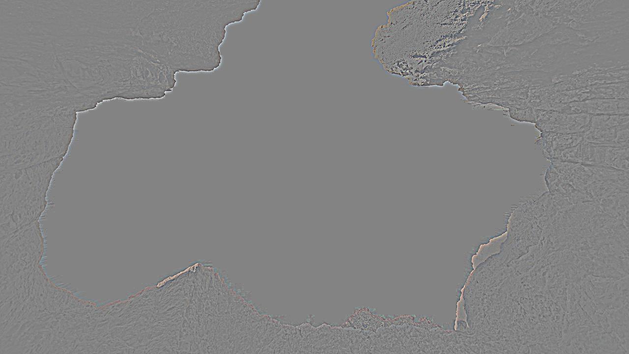
Laplacian stack decomposition for the ocean/mountain blended image


Laplacian stack decomposition for the viewport/everest blended image