CS194 Project 2: Fun with Filters and Frequencies
Part 1.1: Finite Difference Operator
By convolving the cameraman image with finite difference operators D_x and D_y, we computed the partial derivative of the image in x and y.
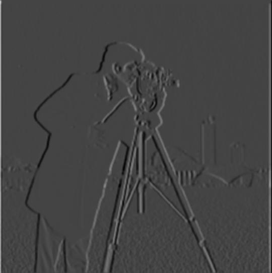
Above is the partial derivative of the image in x.
Above is the partial derivative of the image in y.
After computing the partial derivatives, we then used these values to compute the gradient magnitude image which shows how quickly the image is changing. We can then
use this value to identify the edges because they tend to be areas of greatest change within the image.
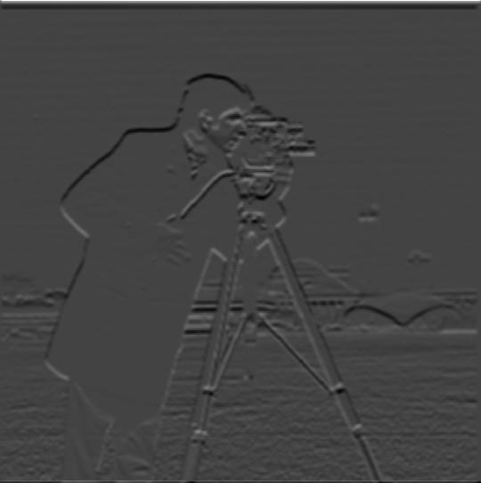
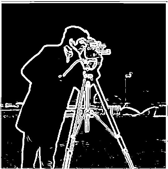
Above is the gradient magnitude image.
After computing the gradient magnitude, I turned it into an edge image by picking a threshold value and changing all values in the gradient
magnitude image that were above that threshold into 1s and the ones that were below into 0s to isolate the edges. After some trial and error, I noticed
that selecting a threshold of 0.25 yielded the best results without too much noise.
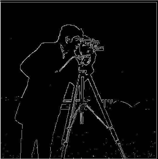
Above is the edge image.
Part 1.2: Derivative of Gaussian (DoG) Filter
The results from the previous part were noisy, so in order to reduce noise, we want to apply a low-pass Filter
to the image to smooth it. We will use the Gaussian filter for this.
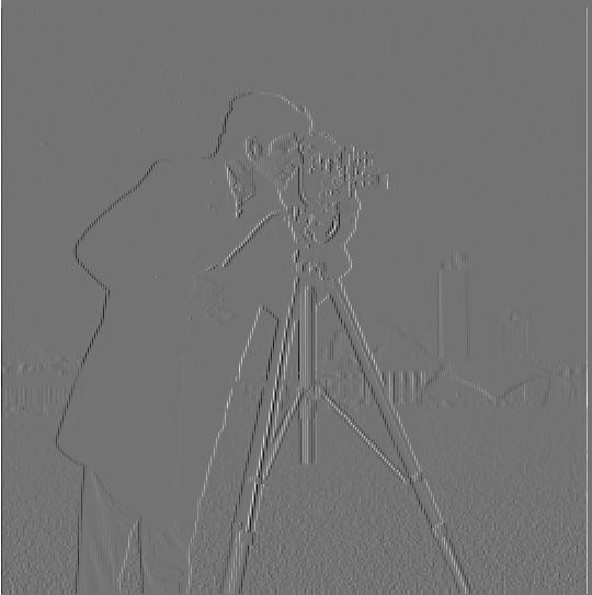
Above is the partial derivative of the image in x with the filter applied.
Above is the partial derivative of the image in y with the filter applied.
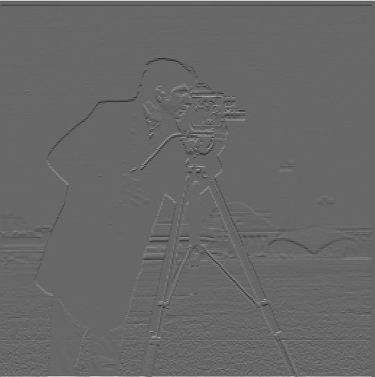
Above is the gradient magnitude image with the filter applied.
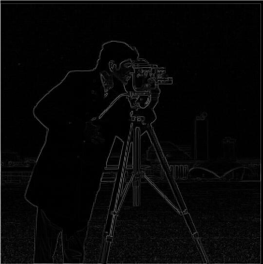
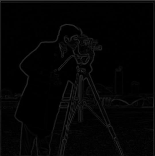
Above is the edge image following the same steps as part 1.1 but with the Gaussian filter applied. We can see that the edges
appear a lot sharper than before, with much less noise. I used a threshold of 0.035. I could use a lower threshold, because the lower
noise frequencies were already filtered out which just leaves us with a much clearer image of the edges.
Part 2.1: Image "Sharpenening"
In this section, we sharpen a blurry image by using the unsharp masking technique. Essentially,
we enhance the higher frequencies, by keeping the high frequencies and subtracting away the low frequencies
we get by applying the Gaussian filter. Through visual trial and error, I decided on a sigma value of 3
for the taj image.
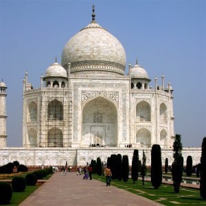
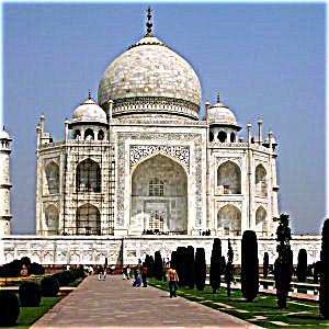
Above is the taj image before any sharpening has been applied.
Above is the taj image after it has been sharpened, most noticeable are that the edges have been sharpened and it looks a little clearer, although
the overall image between these edges still seem a little blurry which is to be expected from this method because we're really only enhancing the higher
frequencies that tend to occur at the edges.
Here, I took a sharp photo, then blurred it then sharpened it in order to compare effects. To blur it, I used the Gaussian filter with a sigma value of
3.
Above is the sharp image before blurring and sharpening.
Above is the sharpened image after being blurred and sharpened with the unsharp masking technique. I used a sigma value of 6 in this case.
We can see that it is still quite blurry, although the edges are sharpened more than the blurred image. This is likely due
to us only enhancing the edges and not addressed the blurry, low frequency pixels in the image.
Here is another image that I sharpened that I found at https://www.shuttertalk.com/fix-a-blurry-picture/
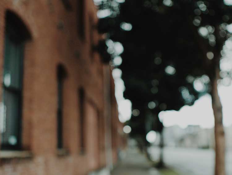
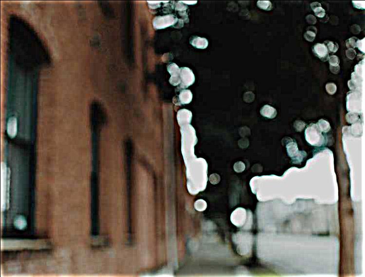
The first is the unsharpened image, and the second is the sharpened image.
Part 2.2: Hybrid Images
In this section, we created hybrid images. These images seem to change when viewing them from different distances. The logic
behind these images is that higher frequencies tend to dominate our vision when they're available, but when we're further away from
the image, we can't see the higher frequencies anymore so we want one image to be composed of the higher frequencies and the other
image to be composed of the lower frequencies.
How I did this, was that I low-pass filtered one image and high-pass filtered the second image (I determined the sigma value
through trial and error for each pair of images), then I averaged the images and clipped them to ensure that the pixel values
were between 0 and 1 before saving the image. I also tried adding the images together, but I noticed that I got better results through
averaging. I noticed that increasing the sigma value of the low-frequency image showed the low-frequency image more since we were keeping more
lower frequencies and filtering out more higher frequencies. And increasing the sigma value of the higher frequency image also showed the image
more because since we were subtracting the blurred image, we would keep more of the higher frequencies and thus would see the higher frequency image
more clearly.
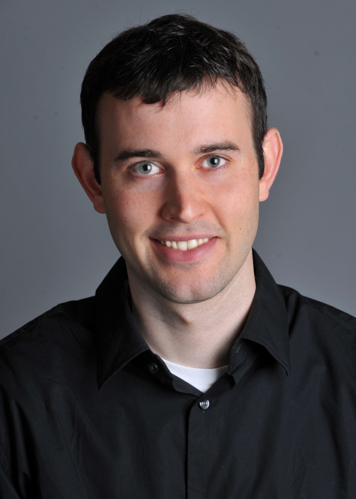
Above is the regular photo of Derek.
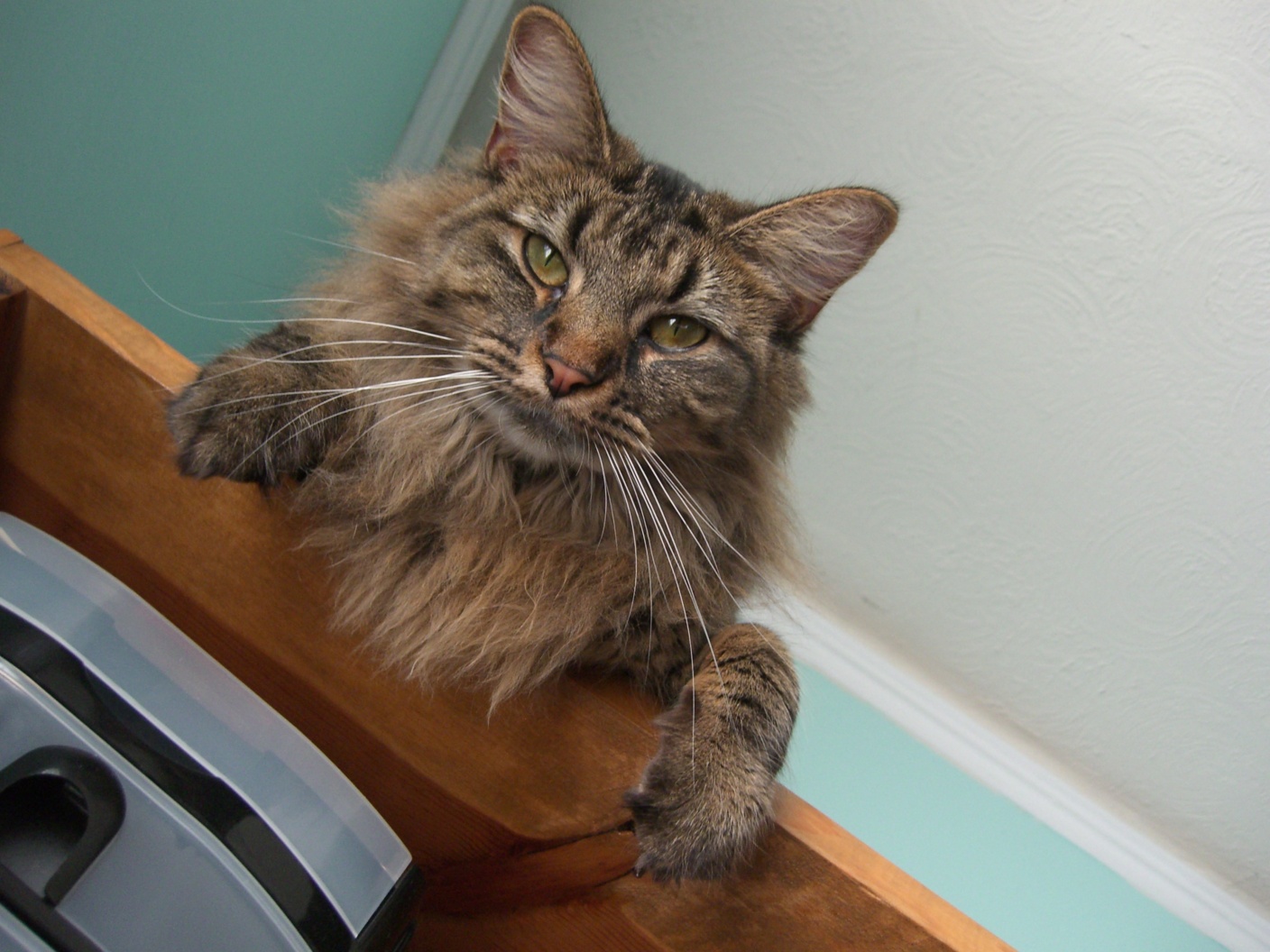
Above is the regular picture of nutmeg.
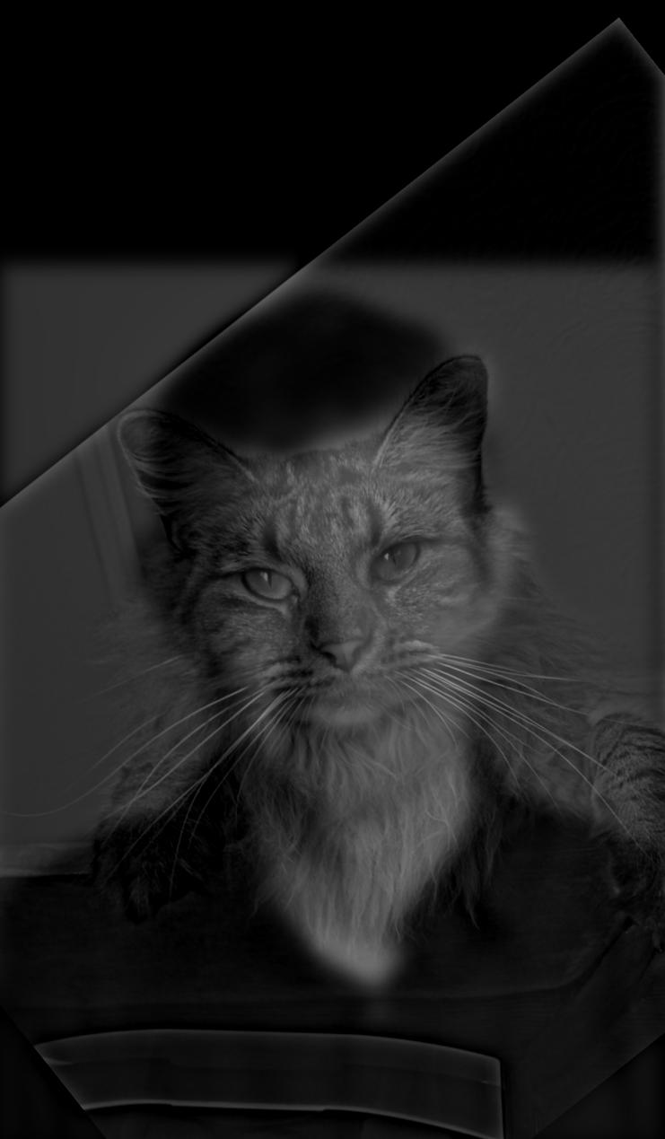
Above is the hybrid image of derek and nutmeg. You can see nutmeg more clearly at a closer distance
and you can see derek more clearly at a further distance.
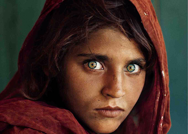
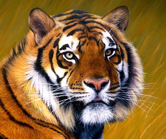
The next image that I used yielded the best results. I blended an image of a girl and an image of a tiger with the tiger appearing at
close distances and the girl appearing at farther distances.
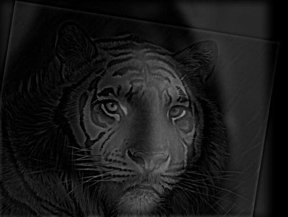
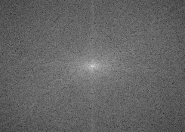
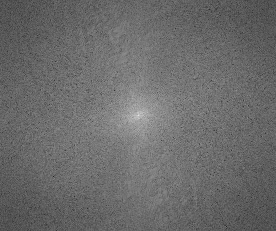
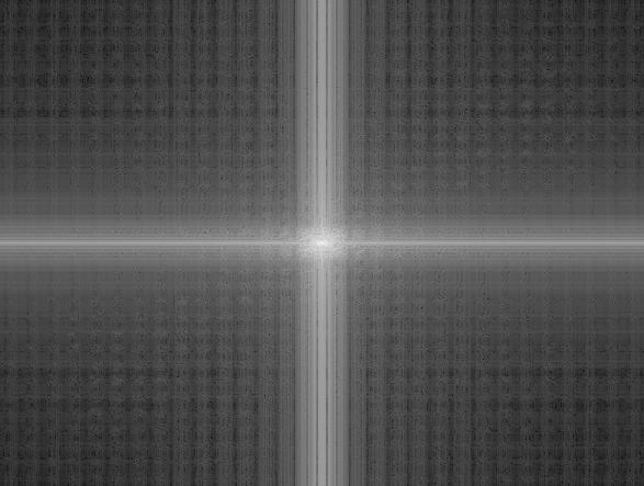
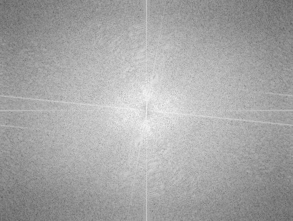
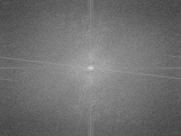
Below, I illustrated the processes of making hybrid images by showing the frequency analysis for the girl/tiger hybrid.
It shows the log magnitude of the Fourier transform of the girl image, the tiger image, the filtered girl image, the filtered tiger
image, and finally the hybrid image.
Below is another hybrid image that I created:
Part 2.3: Gaussian and Laplacian Stacks
In this section, we created Gaussian and Laplacian stacks for blended images.
For the Gaussian stack, I applied the Gaussian filter on the image at each level
with increasing sigma values. I started with a sigma value of 6 and doubled the value
everytime. For the Laplacian stack, I subtracted the respective blurred Gaussian image from the Gaussian
stack, using the same sigma values.
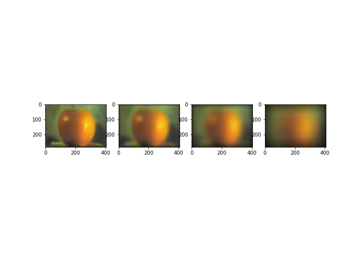
Above is the Gaussian stack of the oraple with sigma values 6, 12, 24, and 48.
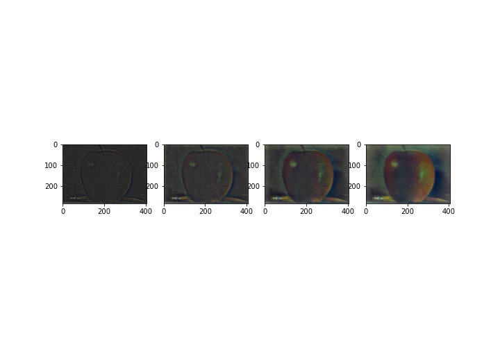
Above is the Laplacian stack of the oraple with sigma values 6, 12, 24, and 48.
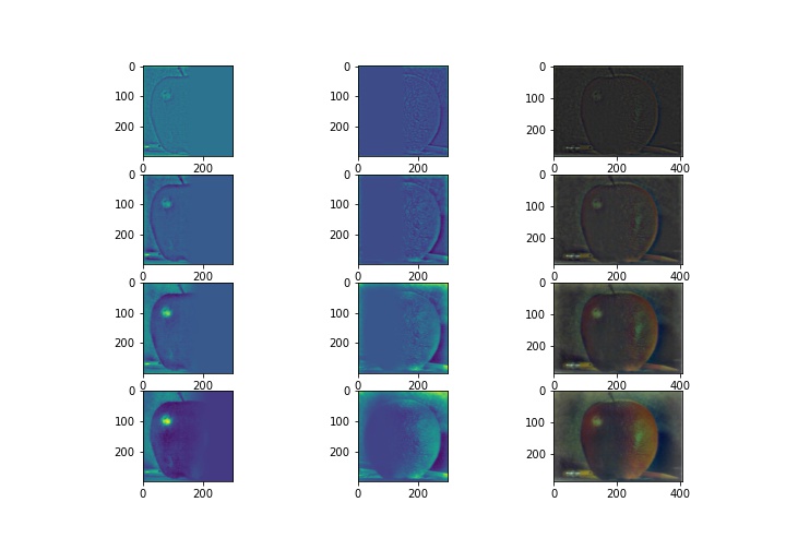
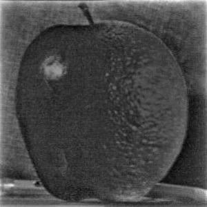
Above is the 12 image figure specified in the spec. It shows the Laplacian stack for the apple on the left and the Laplacian stack for the orange in the middle with the mask used in the next part applied.
In the right-most row, I show the Laplacian stack applied on the blended oraple image.
Part 2.4: Multiresolution Blending
In this last section, we blended the apple and the orange images together to create the oraple.
In order to create the oraple, I took the Laplacian stacks of both the apple and the orange images and also created a mask to blend them.
My mask was a binary matrix with half 0s and half 1s. I took the Gaussian stack of the mask (GR) and at each level, I applied the gaussian stack of the mask
to the laplacian stack at that level of the apple and then took (1-GR) and applied that to the Laplacian stack of the orange at that level.
Once that was done for all the levels, I added all the combined images together to create the blended image.