Fun with Filters

Finite Difference Operator

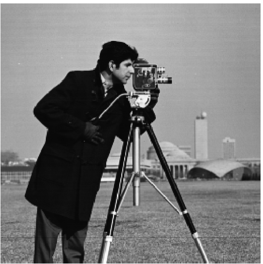
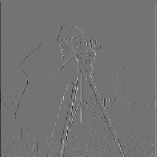
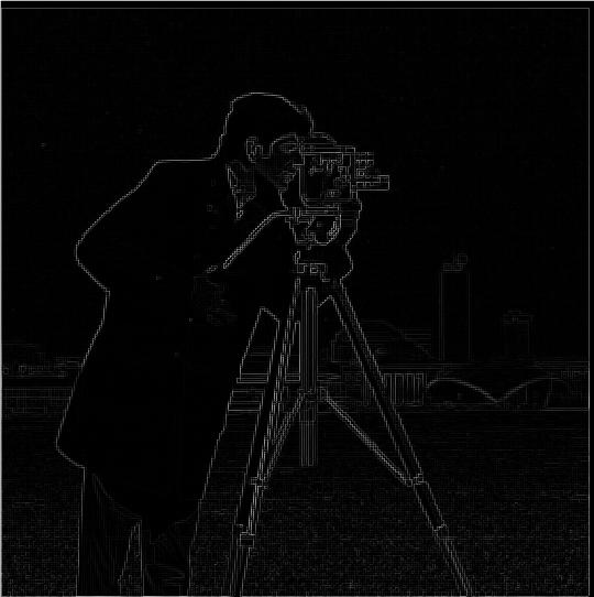
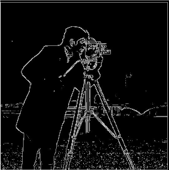
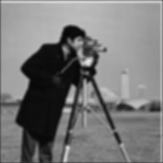
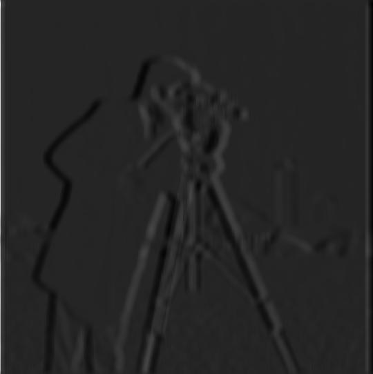
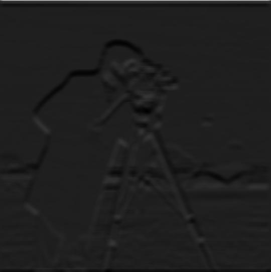
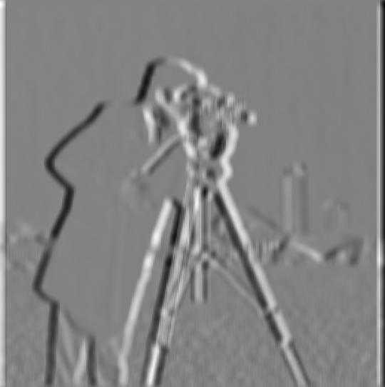
For part 1, I got the partial derivative in the x and y direction by convolving the original image with D_x and D_y. I used the grayscale version of the images to fit the 2d necessity. I then calculated the gradient magnitude image by taking the square root of the sum of the squares of each of the partial derivative images. From there, I used a threshold of .15 to create the binary magnitude image.

Derivative of Gaussian (DoG) Filter

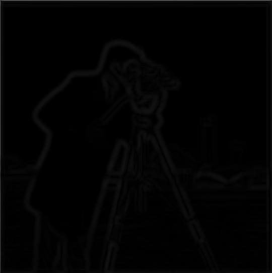
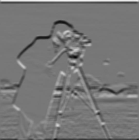
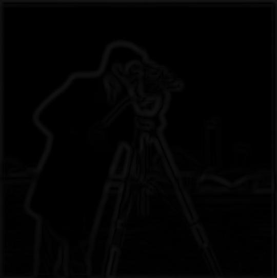
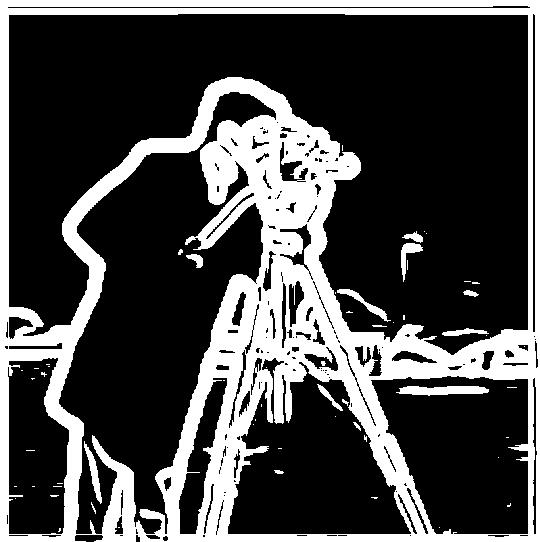
For the DoG filter, I created a gaussian kernel with a kernel size of 15 and a sigma of 5. I took two approaches. In the first approach, I blurred the image by convolving it with our Gaussian kernel and then used the same steps as part 1.1 to get the partial derivative in x and y and the gradient magnitude. I also a binary gradient magnitude with a threshold of 0.01. The results are shown below.

The differences that I see from the pictures below and those we previously got are that the edges are much cleaner and smoother, and they have less noise around the person. We much better capture the edges we desired and extra noise is removed through the blurring process. We get a smoother set of edges that better represent the desired information without losing important details.

The second method is through creating a derivative of gaussian filter by convolving the Gaussian filter with the D_x and D_y filters from part 1.1. We then take these two derivative of Gaussian filters, and we can just convolve these with the original picture to get the partial derivative of the blurred original image. With these partial derivatives, we can find the square root of the sum of the squared partial derivatives again to get the gradient magnitude, and binarize it with the same threshold of 0.01. The results are shown below, and they are the same as the two step blurred edge detector above.

Fun with Frequencies

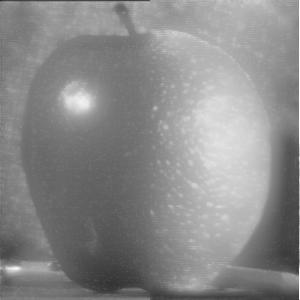
Image "Sharpening"

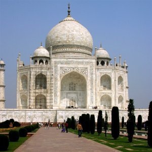
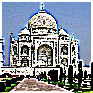
In this section I focused on sharpening images. To sharpen our image, we add on the high frequencies thast we can obtain back into our original picture. To obtain said high frequencies, we use a Gaussian filter to first get our low frequencies similarly to the previous section, and we subtract this with the original image which leaves us with the high frequencies of the image. We just add these high frequencies to the original image with some scaling factor alpha (I iterated through multiple alphas and found 1 to generally perform best) to sharpen the image.

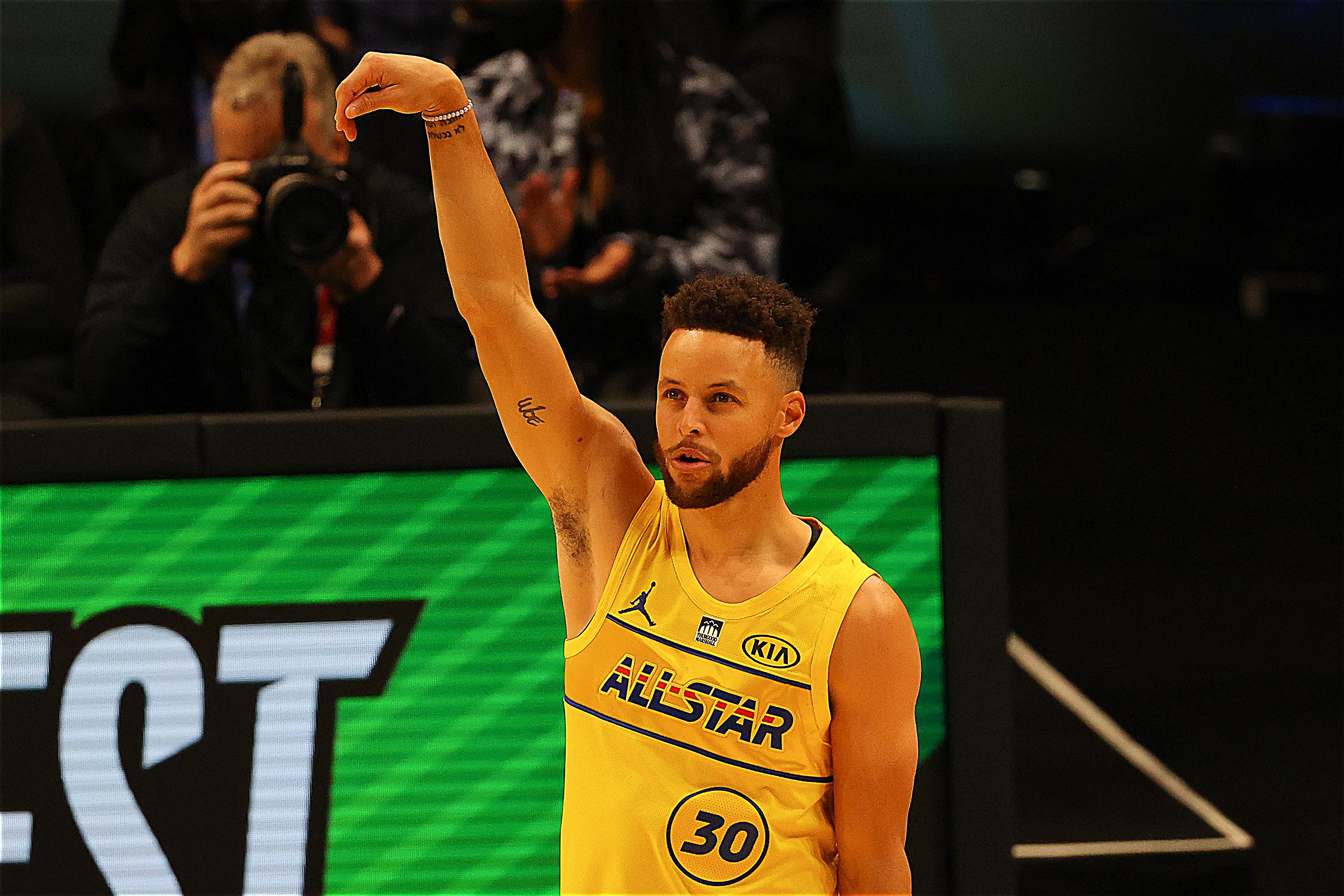
Below are some examples of the original photo and the sharpened photo after. The Taj Mahal's sharpening os very prominent with its edges. The edges look darker and bolded after the sharpening. We can also see the effect of sharpening Stephen Curry with again a focus on how the edges get darker and more defined; however the differences are harder to see.

Next is an example of a picture that was blurred and then resharpened. I blurred everyone's favorite mascot Oski and then resharpened him. The sharpened image is not as good as the original, but is a significant improvement over the blurred image.

Hybrid Images

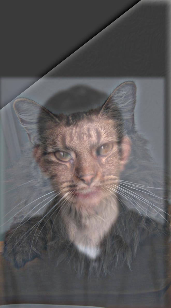
For hybrid images, I first used the given code to align the images. I usually tried to align using the eyes. I then would get the high frequencies of one image and the low frequencies the second image and average them together into a single photo. This photo would be the hybrid image that looks like the high frequencies up close and the lower frequencies from a distance. I iterated over multiple sigma values to find the optimals for each photo.

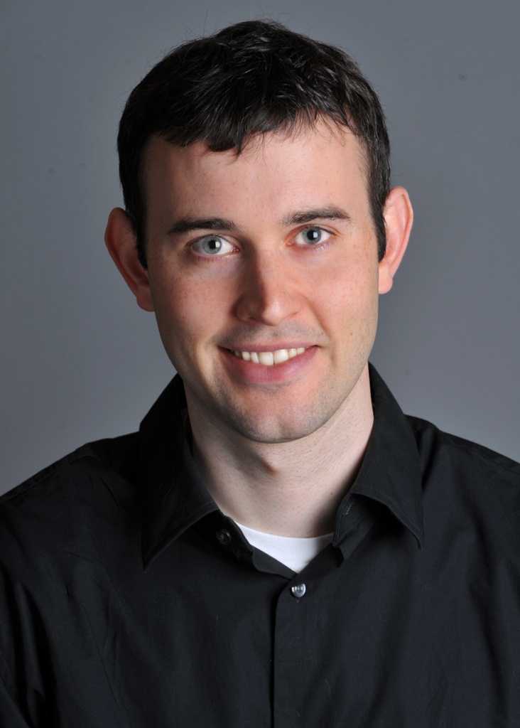
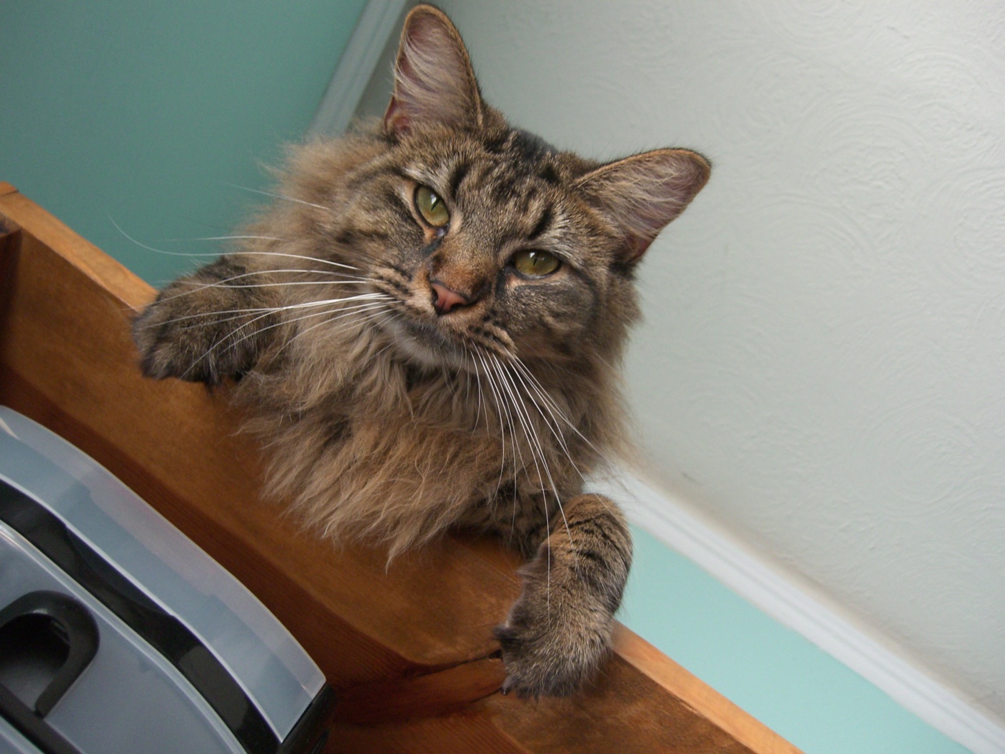
Below is Derek and nutmeg in hybrid form.

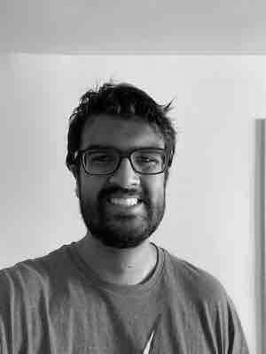
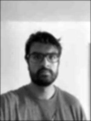
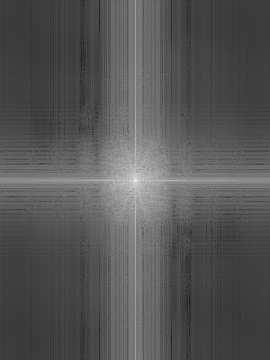
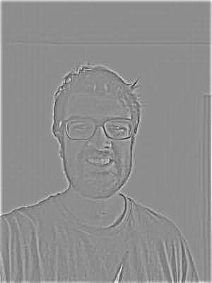
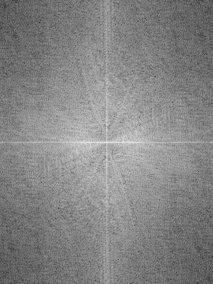
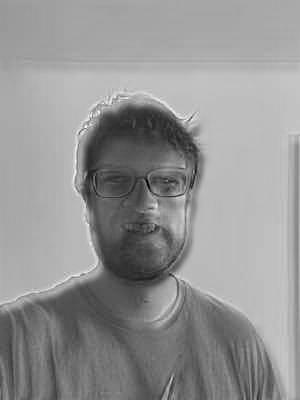
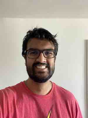
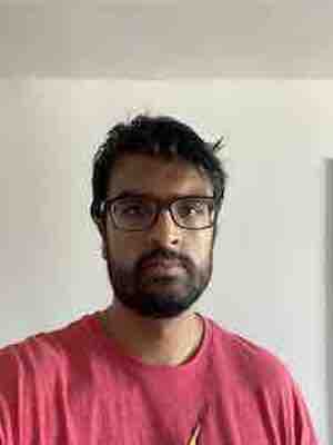
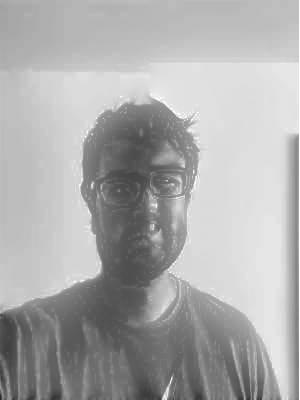
Bells and Whistles I made a color image for the low and the high frequency. For later parts, I used grayscale images. For the background image, having color adds value as it makes the photo seem more realistic from afar and differentiates a bit more from the high frequency iumages. The high frequency image may actually be better in grayscale as it starts to conflict with the low frequency image when in color.

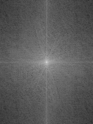
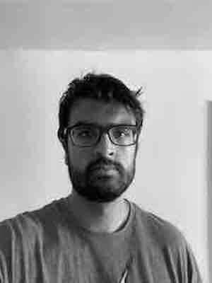
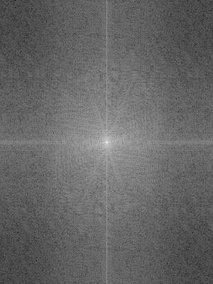
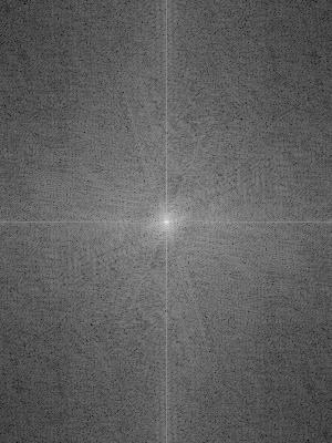
Here is a picture of me looking happy and mad (kind of) with their respective frequencies. We see with the frequencies that many of the happy me's high frequencies were removed, making the low frequencies seem wider and more visible and the mad me's Fourier image brightened on the axis, which showed that we only have the high frequencies now. The hybrid fourier looks like a normal image because have the low and the high frequencies. It is not as bright as the high frequency mad me and has more high frequencies than the low frequency happy me.

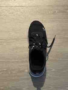
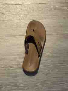
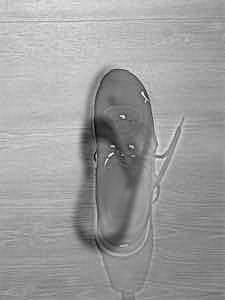
Below is an example image that does not work as well as we would hope. It combines a flipflop and a shoe, but the overlap and alignment force the image not to overlap well causinga weird looking photo that does not have this cool "becoming" another item effect. However, from far the image does look more like a shoe and from close the flip flop is visible.

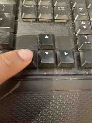
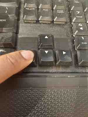
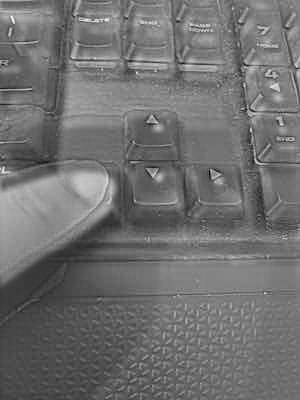
This example does better as we see me clicking a key on the keyboard.

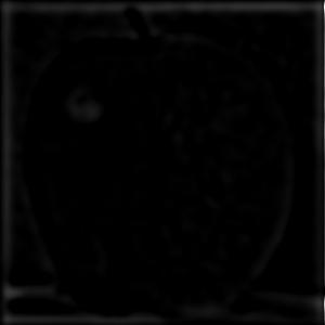
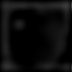
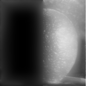
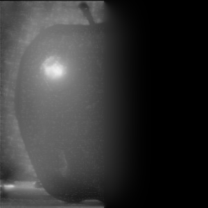
Gaussian and Laplacian Stacks

For this section, I blended together images. I first created a Gaussian stack. To get the Gaussian stack, I blurred each picture with a Gaussian filter. The first picture in the stack is the original, and each picture after is a Gaussian blur of the previous picture. Additionally, as the stack increased, the sigma value increased. Each sigma value was 2^i, where i is the index of the image that is blurred. I started with sigma = 2.

I then ceated a Laplacian stack. To make one, I subtracted each immediate pair of pictures. I also added the lowest frequency picture in the Gaussian stack to the end of the Laplacian stack, so it would be easy to just sum the Laplacian stack. I then followed the procedure in the paper to reconstruct the image.

Here is the recreated figure 3.42 in color. (I used additional levels)

Multiresolution Blending

To create this process, I created a mask. For the oraple, it is just a binary mask with 1's on the left side and 0's on the right side. I created a Gaussian stack with this mask to make sure there is blending in the middle. I then multiplied the orange Laplacian stack with the mask Gaussian stack level by level and element by element. I also multiplied the apple Labplacian stack by one minus the mask Gaussian stack level by level and element by element to get the left side of the apple. I would then sum together each half together for each level. Finally, I sum together the whole stack to get back the blended picture.

For regular mask, I tried blending my happy and mad faces from before. It led to an interesting result. While the tops of the heads did not align, the rest of the body merged well creating a very demented me.

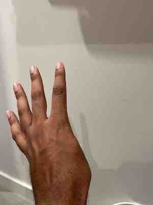
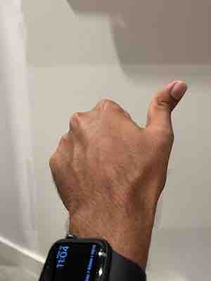
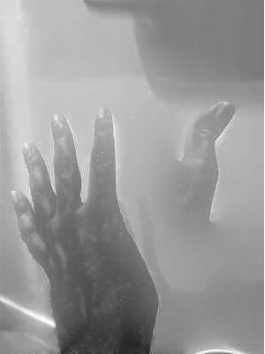
For an irregular mask, I tried to create an impression that my thumb came off my hand. To do this I tried to only capture the top right of the image that contained my thumb, thus using a filter that only captured that section instead of the entire right half. This is the eerie result: