Overview

This project aims to explore different manipulations of filters and frequencies including edge detection, blurring and sharpening, creating hybrid photos, and merging different into a single image. The results of the required and personal exploration of these manipulations are detailed below along with images to further illustrate what was done for each subsection of the project.

Part 1: Fun with Filters

Part 1.1: Finite Difference Operator

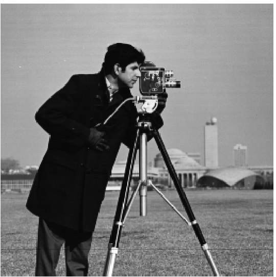
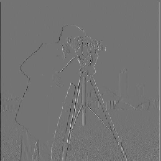
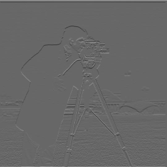
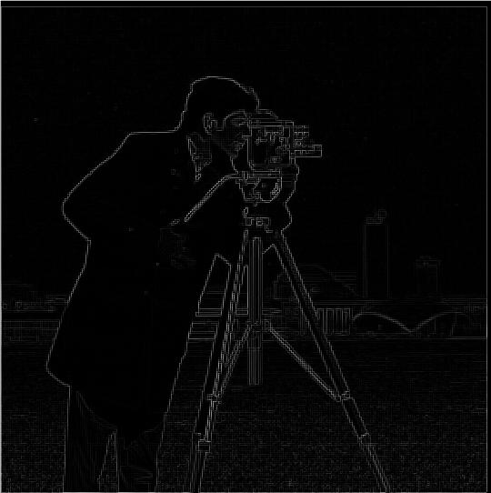
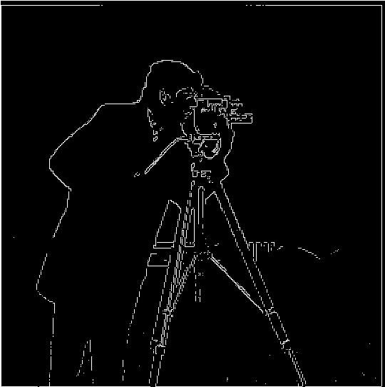
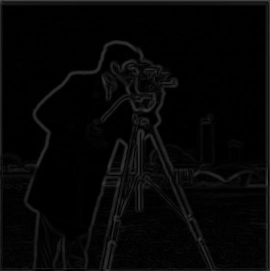
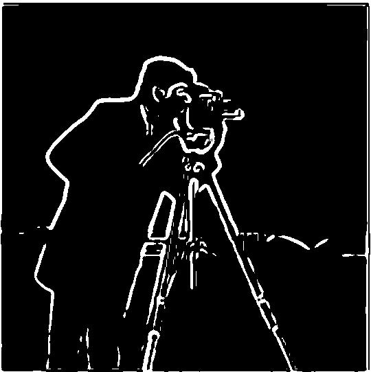
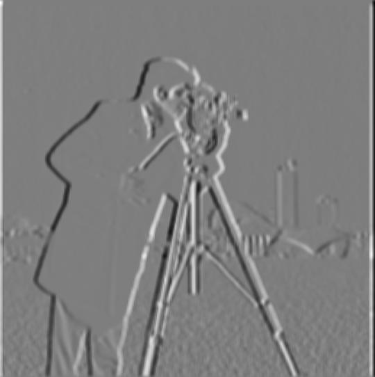
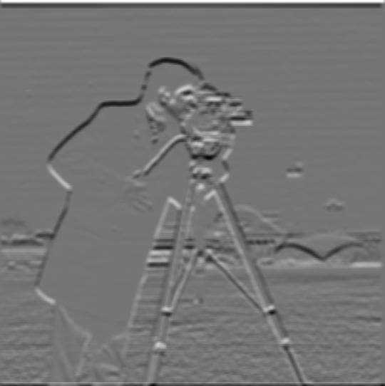
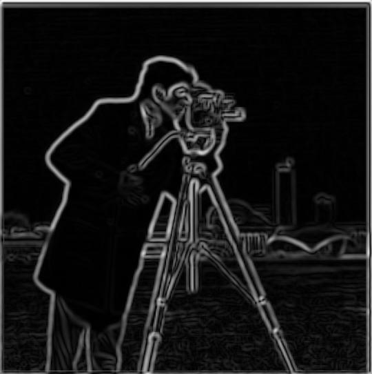
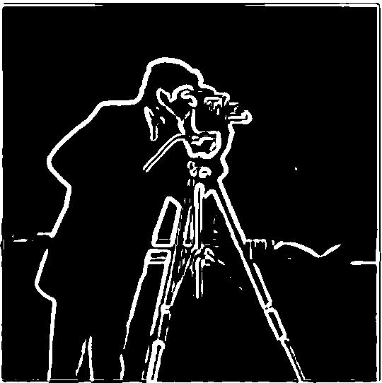
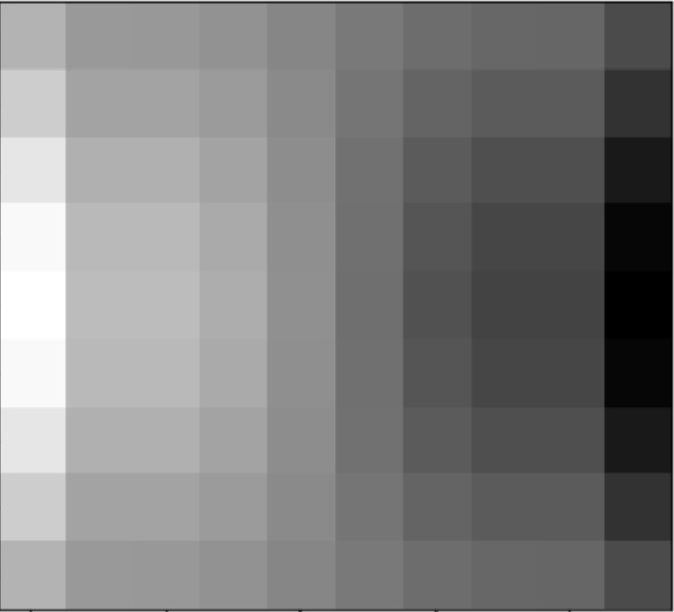
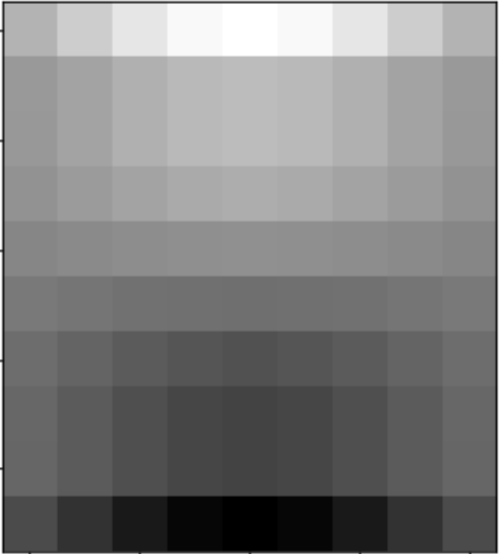
In this part, we derive the partial derivate images of the cameraman. This is done by convoluting the image with finite difference operators (convolve2d). The gradient magnitude image is then calculated by squaring both partial derivatives, adding, and at last square rooting the sum. The gradient magnitude image is in effect an edge detector. To filter out some noise a threshold is selected to binarize the edge detection (above = 1, below = 0). The results are shown below.

Part 1.2: Derivative of Gaussian Filter

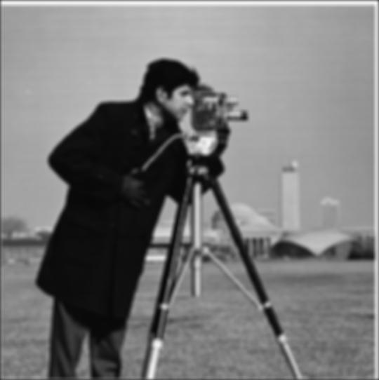
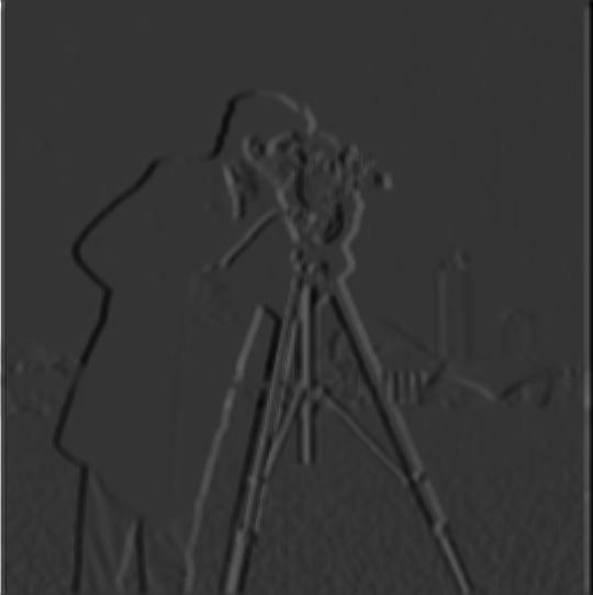
To cut out some of the noise from the previous part, we use a gaussian filter to smooth out the image before preforming the convolution with the finite difference operator. This provides a much more pronounced edge image with less noise.

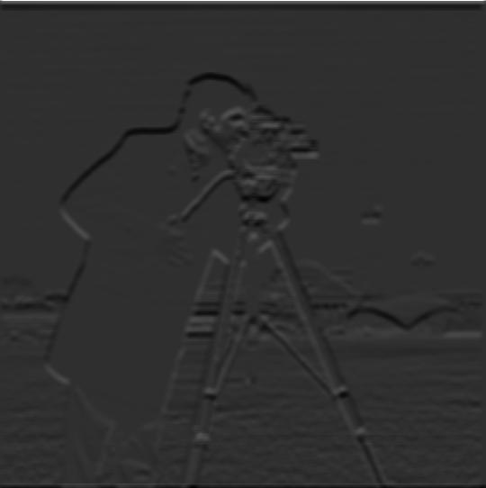
To further simplify the process, the gaussian blur and finite difference operator can be applied by first convoluting the partial derivative with the gaussian filter. Then applying the resulting DoG filter to the image itself. The results below differ vary little from those above. Note: the main difference between these images is the magnitude of the pixel values (one is brighter than the other). Aside from that, the results match.

DoG Visualization

Part 2: Fun with Frequencies

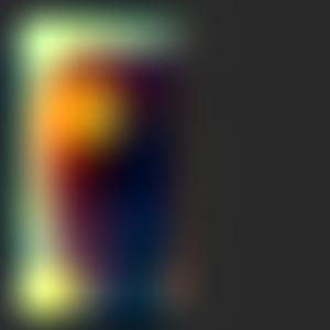
Part 2.1: Image Sharpening

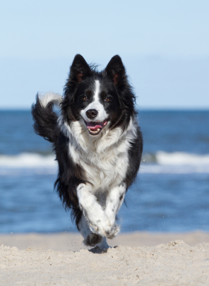
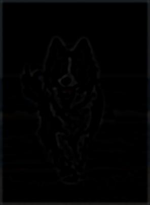
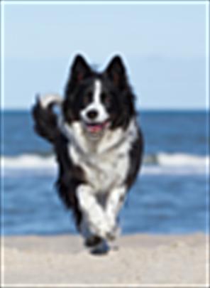
To sharpen an image, the higher frequencies of an image need to be emphasized. To isolate the higher frequencies we use a low pass filter (Gaussian blur) to first eliminate the high frequencies. Once this is done, we can then subtract the blurred image from the original, thereby leaving the higher frequencies present. This effectively detects edges or areas of stark contrast but retains little of the original image. We then multiply this high pass filtered image with a constant alpha and add to the original image. This emphasizes the higher frequencies and "sharpens" the image.

The next set of dog images undergoes a slightly different process. The blurred image is passed in as the original image and sharpened. The results differ significantly as there is a loss of high frequencies when we attempt to sharpen a blurred image due to the image already having been low pass filtered. Thus, even with an alpha value of 2, it is a far cry in terms of "sharpness" from the original image.

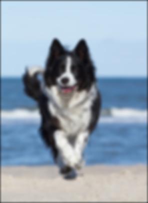
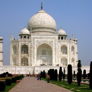
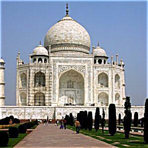
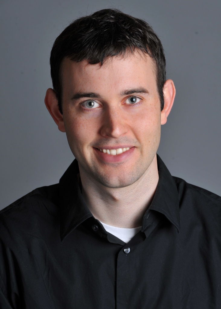
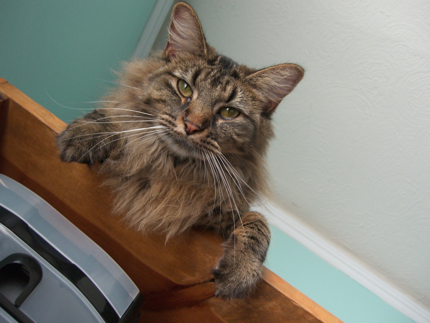
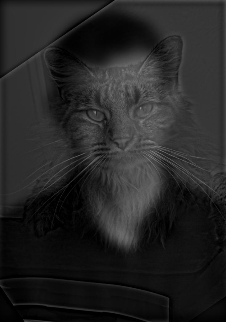
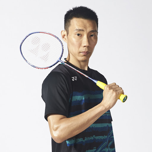
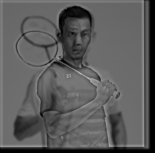
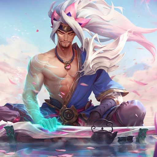
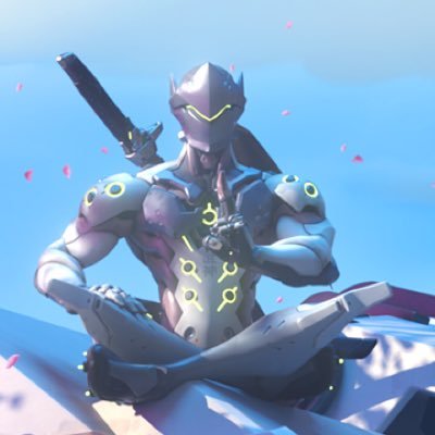
Part 2.2: Hybrid Images

This next section explores an interesting concept regarding higher and lower frequencies in a single image. Hybrid images incorporate two aligned images into a single picture. This is done by combining the low frequencies of one image with the high frequencies of another through a simple pixel by pixel averaging of the isolated low and high frequencies. Once again, the lower frequencies are isolated with a gaussian blur and the high frequencies isolated by subtracting a gaussian blurred image from the original. The viewer can then only clearly perceive the high frequency image at close distances and the low frequency image at farther ones. The images below were created through the above process with varying sigma thresholds (Gaussian blurs) due to each pair of images unique attributes.

An important aspect of creating hybrid images is the alignment. Because the low frequency image can be seen through high frequency image at close distances it is important that the images are aligned in a fashion that will not make the images conflict too much. As you can see from the images above, the images were selected such that the objects/people in the photos have more or less the same pose.

Failure Case

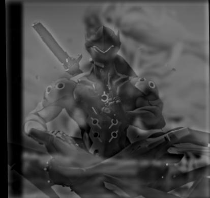
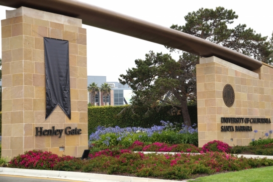
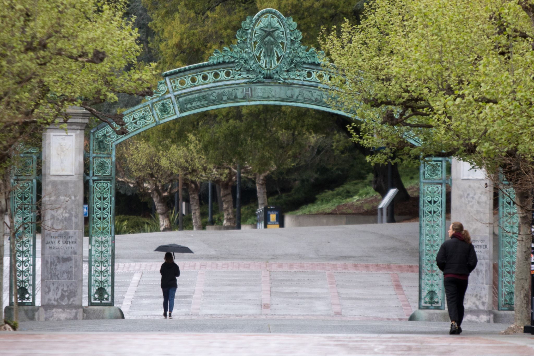
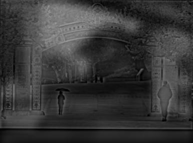
The case below attempts to create a hybrid image with some gates from UCSB and UCB that do not exactly align since they are from compeletely different angles. It is apparent from this image that alignment is important as it is difficult to associate the background details with the UCB image at close distances. Overall, the Berkeley image is difficult to view even at closer distances.

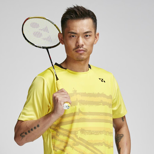
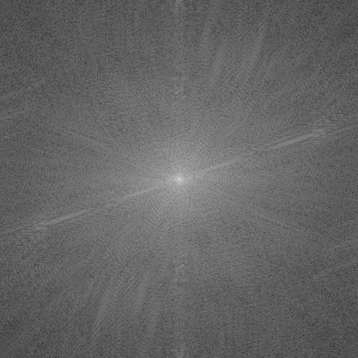
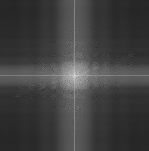
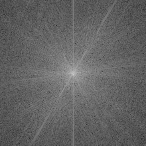
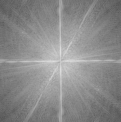
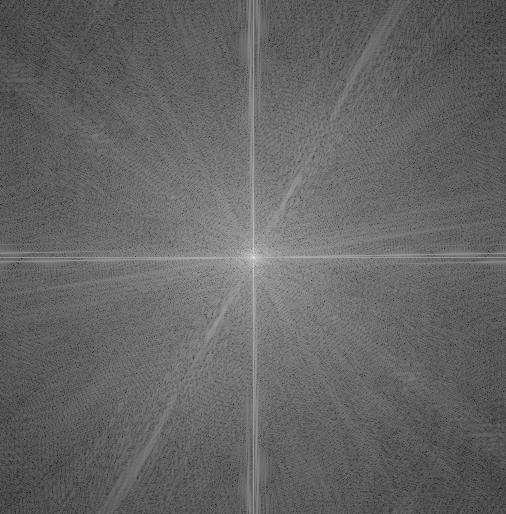
Fourier Representation

We can observe the creation of the hybrid images through a different image representation: Fourier Transforms. In this representation, higher frequencies are represented as dots farther from the center of the image, while lower frequencies are towards the center. Below are the original Fourier representations of the Lin Dan and Lee Chong Wei hybrid image process, the post-filter representations, and final hybrid image representations.

Part 2.3: Gaussian and Laplacian Stacks

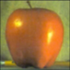
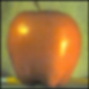
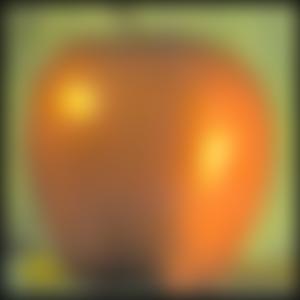
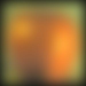
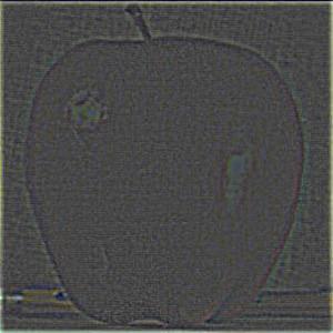
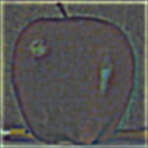
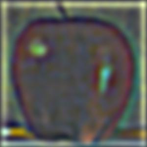
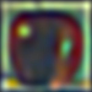
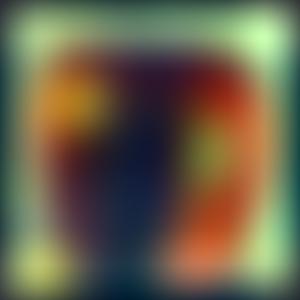
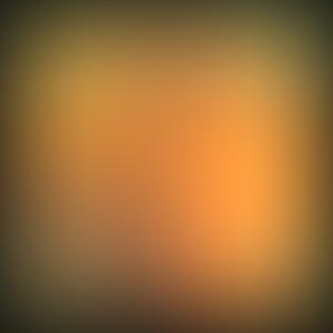
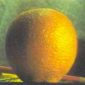
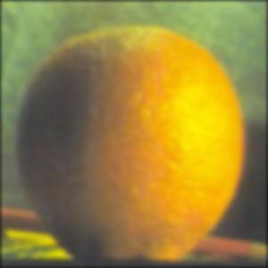
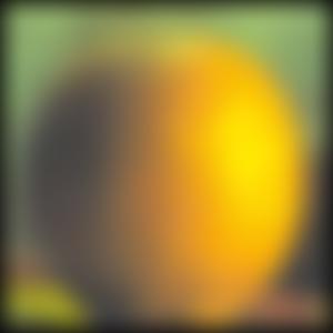
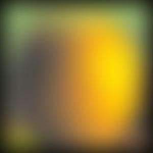
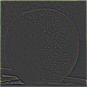
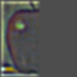
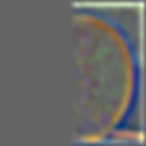
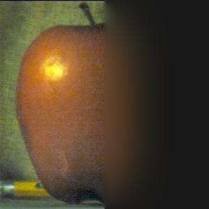
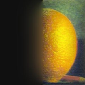
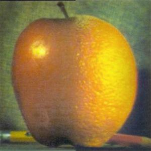
Both Gaussian stacks and Laplacian stacks are stacks of images with the same dimensions but contain a different distribution of frequencies across the board. Gaussian stacks are formed by repeatedly applying a larger and larger gaussian blur at each level of the stack. At the highest level, we apply a G(9,3) blur. Each level down we double the sigma value and therefore the size of the Gaussian filter. Laplacian stacks take the aforementioned Gaussian stack and process the layers like so: L(i) = G(i) - G(i+1). By subtracting one layer of the Gaussian stack from the other, we create a band-pass filter. Thus, each level of the Laplacian stack contains a different band of frequencies which can be collapsed to reproduce the image. The last layer of the Laplacian stack is the last layer of the Gaussian stack. Below are the Gaussian and Laplacian stacks of the apple and orange images in preparation for alpha blending in the next part. 6 layers were used.

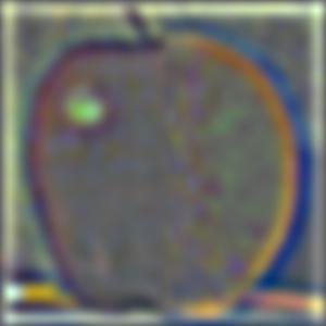
Part 2.4: Multiresolution Blending

In this last part of the project, we use the Laplacian stacks from the last part and some newly created Gaussian stacks to blend the apple image with the orange (oraple). We begin by first creating an alpha mask with half ones and half zeros as our intention is to create the oraple by merging the apple and orange at the middle. This alpha mask is then passed in the Gaussian stack function and treated the same way as any image channel in the previous part. Once this has been done, we can begin merging. At each level of the Laplacian stacks, the alpha mask at the same level is "applied" to both the apple and the orange images (orange uses 1 - alpha to get the other side of the oraple). These images are then added. The result is a 6-layer stack with the alpha applied merged images at each level. The last step before displaying the final oraple is to collapse the stack by adding all the layers. The results of the process is shown below mimicking that of the research paper.

Other Blending Attempts

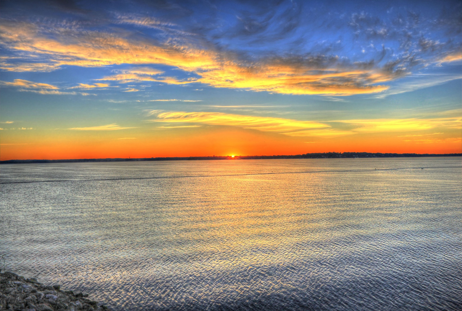
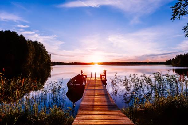
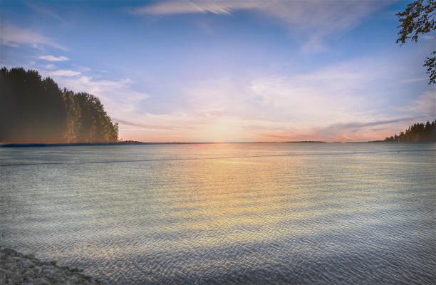
The following set of images utilizes the horizon in 2 lake images as the boundary for the merge instead of a vertical boundary like with the oraple case.

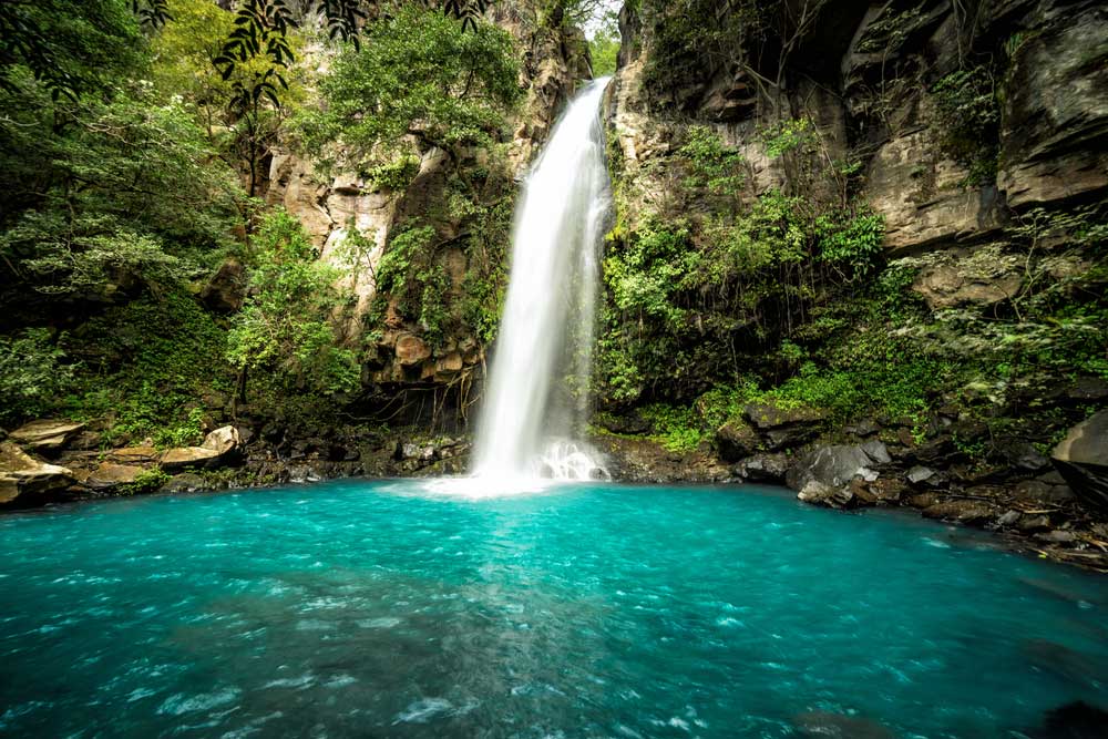
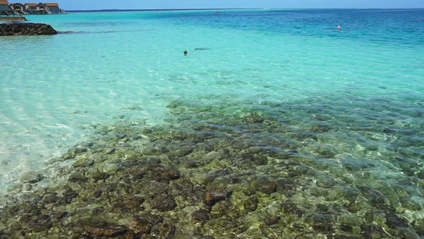
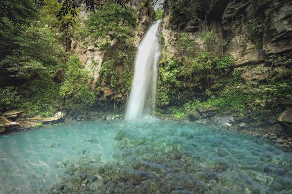
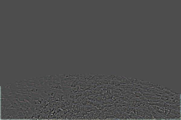
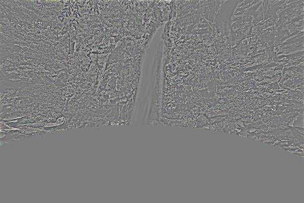
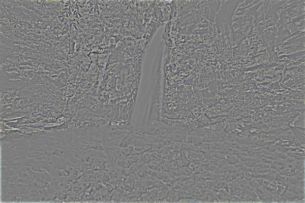
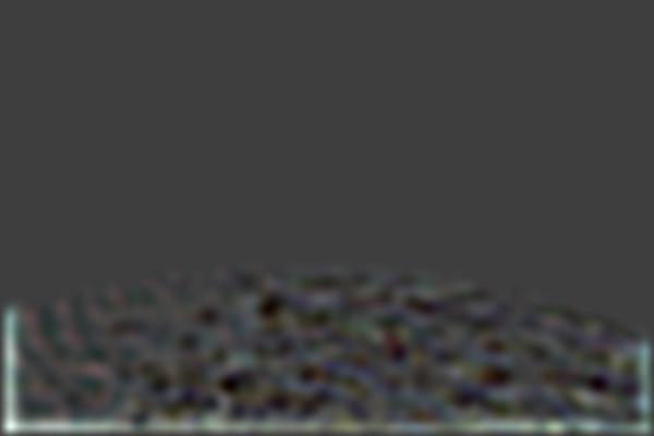
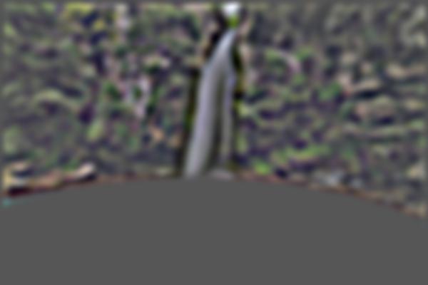
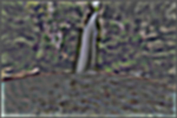
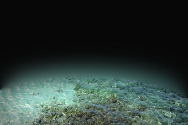
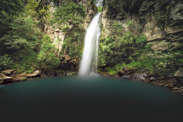
The next set of images are the result of using an irregular mask. This one was constructed using the equation of an ellipse to encompass the water below the waterfall and replace it with that off a coral reef.

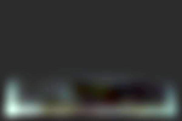
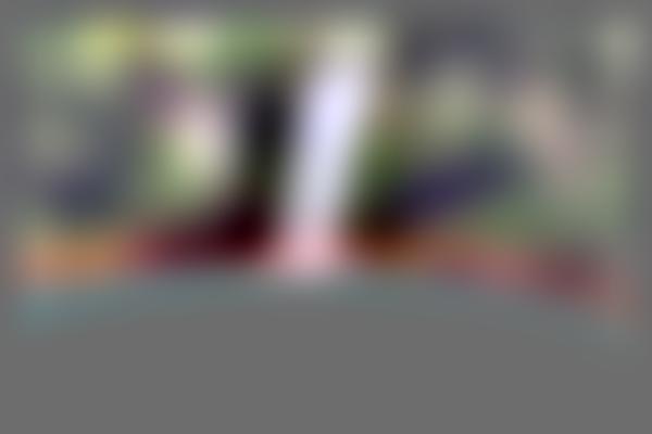
Here are the Fig 10 style images for the Ocean/Waterfall blended image.

Conclusions

The most interesting thing I learned from this assignment is really everything from this project. I feel that I have a decent amount of interaction with photo editing software including Photoshop and Procreate. However, even with that experience, understanding what's is really under the hood for the more popular operations such as the gaussian blur and smoothing tools really shines a different light on those softwares. It may even help in utilizing those tools better for photo editing/creating purposes.