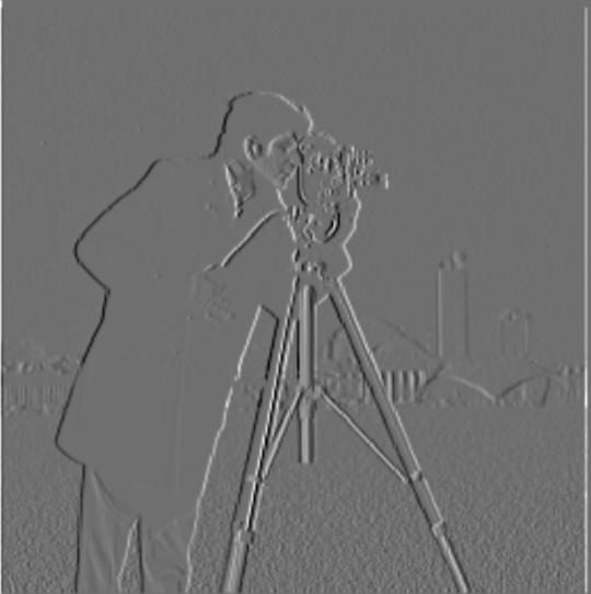
In this part, we used the finite difference filters of Dx = [1 -1] and Dy = [1 -1]^T in order to compute the magnitude of the gradient in the horizontal and vertical directions respectively, giving us gradient_x, and gradient_y.
We then computed the overall gradient via the formula gradient = sqrt(gradient_x^2 + gradient_y^2).
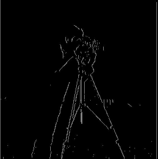
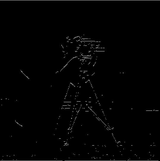
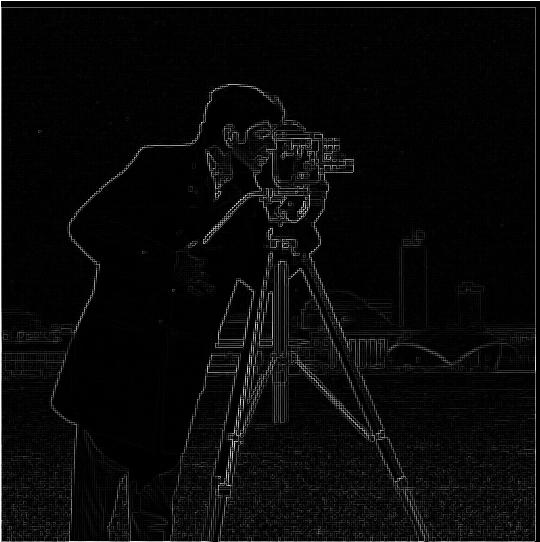
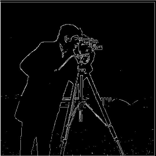
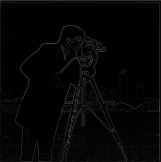
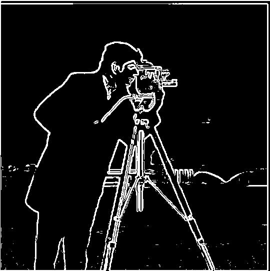
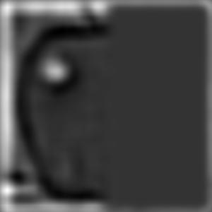
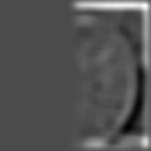
The images below are the partial derivative wrt x, the partial derivative wrt y, the gradient of the image, and the binarized gradient of the image (in that order).
In this section, we used the gaussian filter to blur our original image, then took the finite difference operators over the blurred image. We then formed DoG filters by convolving the finite difference operators with the gaussian, then convolving those filters with our images.
This approach yielded much clearer edges than we saw in part 1.1, since we avoided having to threshold out some amount of noise by blurring the image before taking the partial derivatives.
Results with the DoG filters were the same as those we got by separately blurring the images, and then taking the partial derivatives of the blurred images.
These are the DoG filters for x and y (in that order).


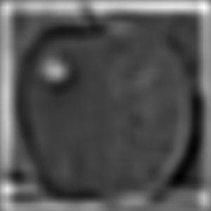
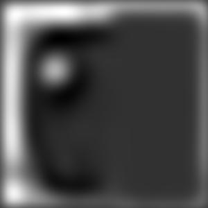
These are the results of convolving the DoG filters with the original cameraman image. The images are in the following order: partial derivative wrt x, partial derivative wrt y, gradient magnitude, binarized gradient magnitude.

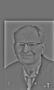
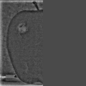
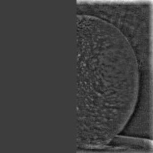
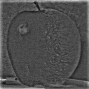
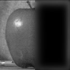
We can sharpen images by amplifying the high frequency components of the images. We do this by taking a gaussian filter over the image to blur it, then subtracing the resulting low frequency features from the original image to get the high frequency features. We can then scale and add these high frequency features to the original image to get a sharpened version of it. The results of this approach are below. The original image is displayed first, followed by the image sharpened with alpha = [1, 2, 5] in that order.
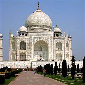
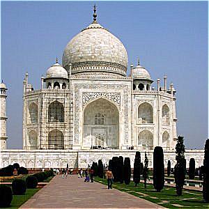
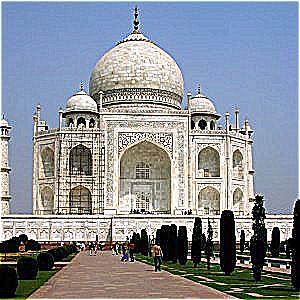
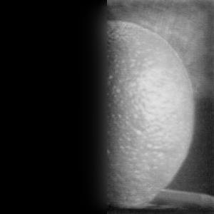
We can combine the operations from the naive sharpening approach into a single convolution operation called the unsharp mask filter. Given an image f, a scaling factor alpha, the unit impulse e, and a gaussian filter, the unsharp mask filter is given by ((1 + alpha)*e - alpha*g). Convolving this with our image f gives us the sharpened version of our image, as in the previous section. Below are results for blurring a sharp image, and resharpening it using the unsharp mask filter. The original image is displayed first, followed by the blurred image, followed by the image resharpened using the unsharp mask filter.


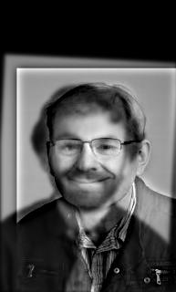
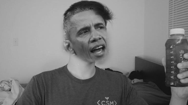
This one looked pretty weird because their heads were different sizes in the images, and somehow looks like neither of them.

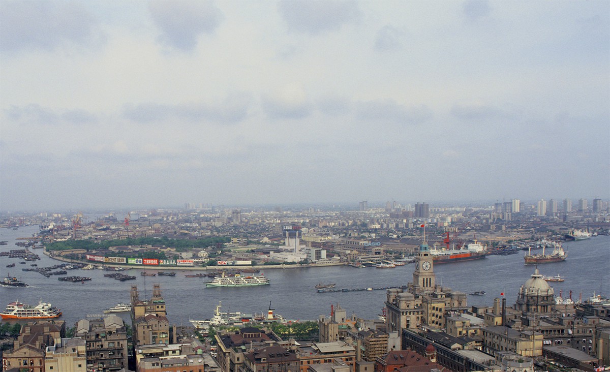
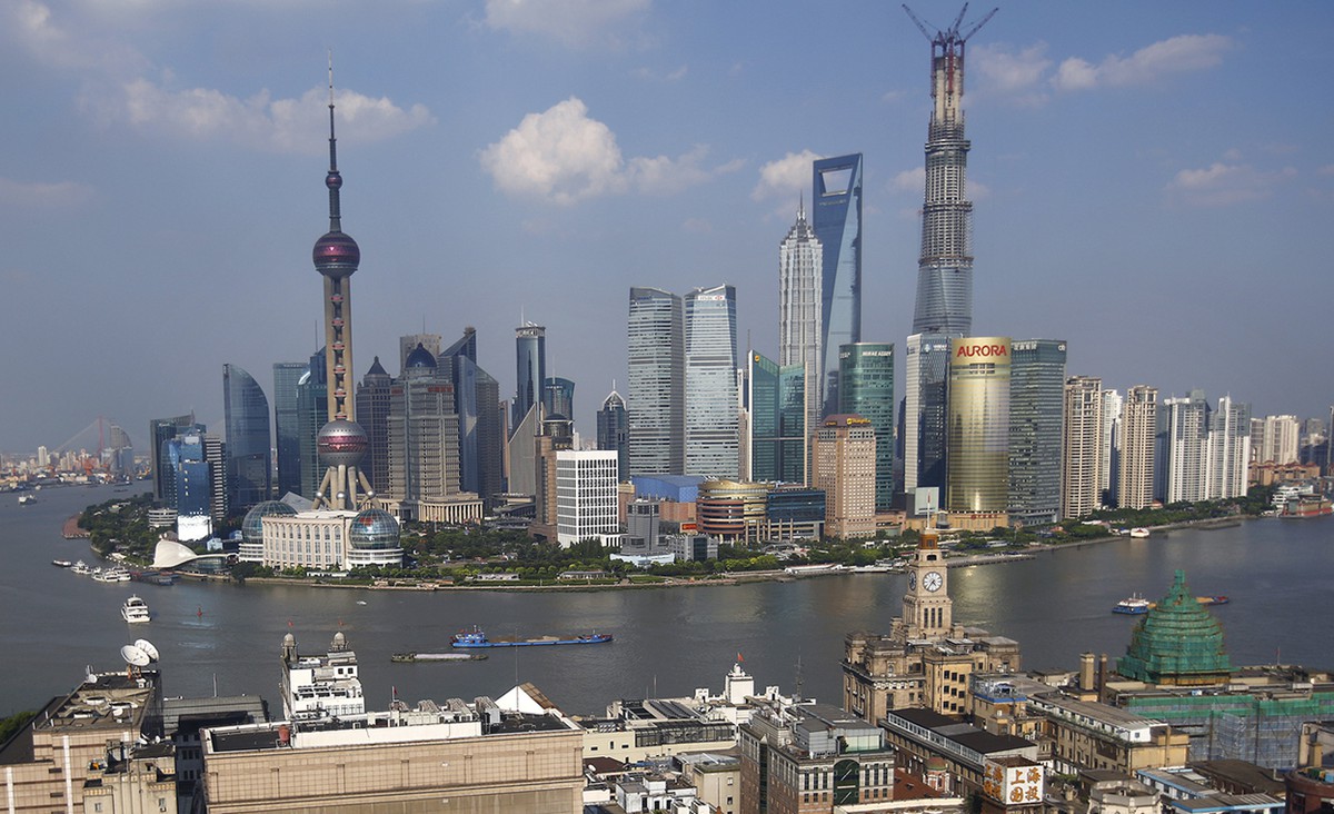
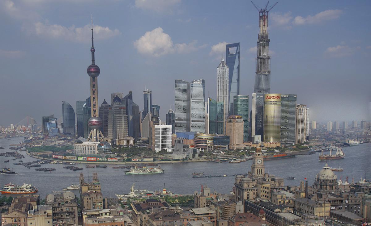
I thought that the multiresolution blending using the laplacian stacks was really cool - I really liked the output of blending shanghai then vs now, and playing around with the mask to get a nice looking output. The use of frequencies for hybrid images was also really interesting, and very important in understanding how we percieve different levels of features in images differently. I also learned that it's pretty hard to align images and get them to be the same size for transferring their features to other images.