This project is focused on developing filters and manipulating images by manipulating the frequencies of the images. In particular, we first use a finite difference operator and a derivative of Gaussian filter to detect edges. Then we amplify the high frequency portions of images to "sharpen" them (unsharp mask filter). Similarly, we combine the low frequency and high frequency portions of two images to form hybrid images. Finally, we implement multi-resolution blending using Gaussian and Laplacian stacks.
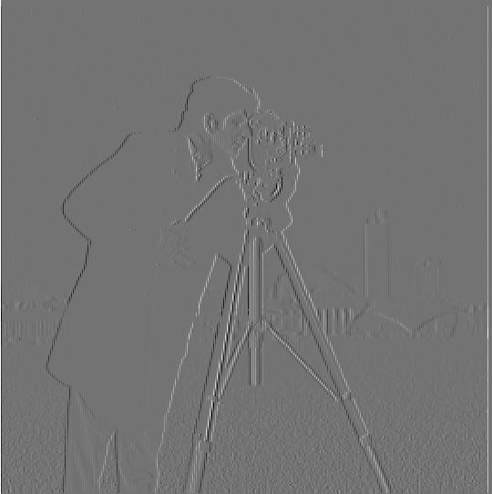
I convolved D_x and D_y with the cameraman image. Here is the result:
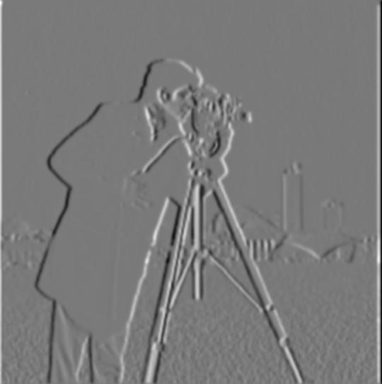
The partial derivative in x:
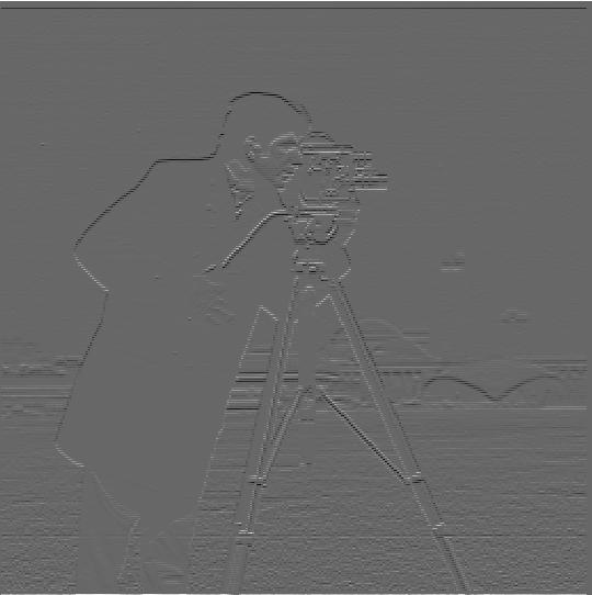
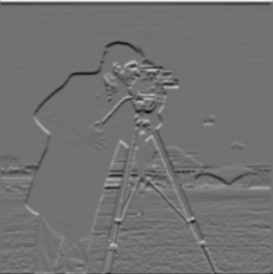
The partial derivative in y:
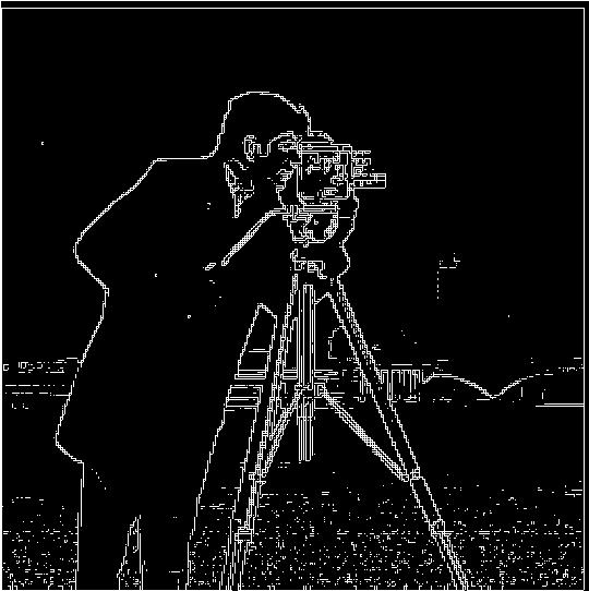
For the gradient magnitude, I used the formula from the slides. That is, final_img[i,j] = sqrt(dx[i,j]^2 + dy[i,j]^2). In the code, I use a vectorized form using numpy methods. Hers is the result:
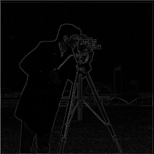
Currently a bit dark but if we threshold the image, we get:
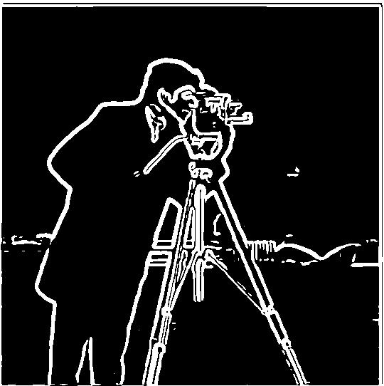
First, we take a blurred version of the cameraman and run the finite differences method on it.
"What differences do you see?" - The edges are much smoother. A lot of the noise in the cameraman binarized image from part 1.1 is removed. It seems more of a natural edge detection when compared to part 1.1 which seems significantly more pixelated. The image that is produced when convolving with the DoG filter is the same as applying the Gaussian before the finite differences operation (as expected).
For the DoG filter, I first convolved the 2D Gaussian with Dx and Dy.
Gaussian Dx:

Gaussian Dy:

Then we can see the image convolution with Gaussian Dx and Gaussian Dy:
Cameraman Gaussian Dx:
Cameraman Gaussian Dy:
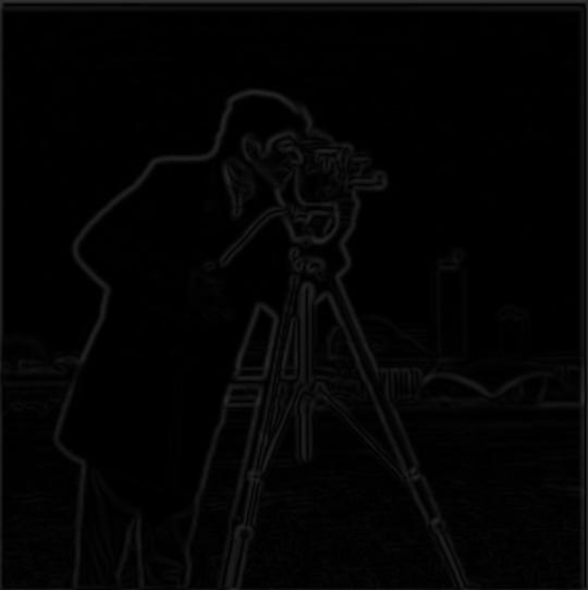
The gradient magnitude computed the same way as part 1.1:
Cameraman Gaussian Dx:
Binarized gradient image
"Verify that you get the same result as before." They're the exact same. Here is the result when applying the Gaussian to the image and then running finite differences:

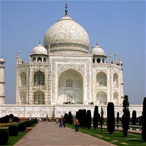
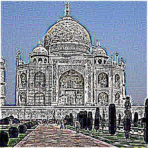
For the image sharpening, I used the formulation that only applies one convolution. (i.e. the formula with the unit impulse.) First, I show the results on the Taj image.
Sharpened with Alpha=0.4:
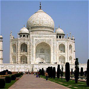
Sharpened with Alpha=1:
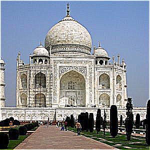
Sharpened with Alpha=5:
Sharpened with Alpha=50:
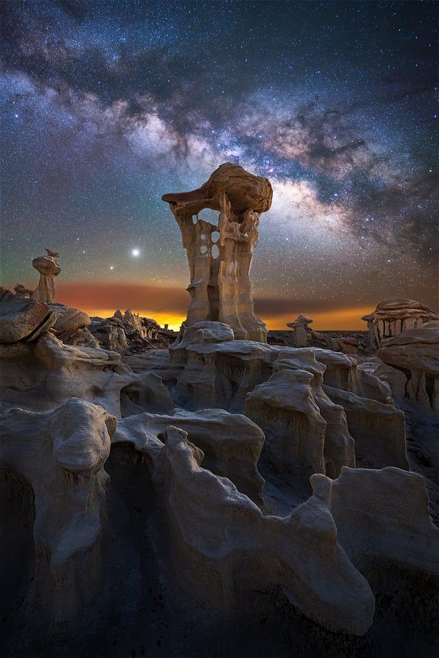
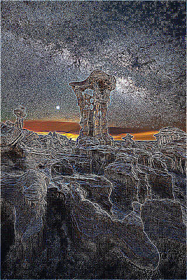
I also use two different images to show the process. First is an image of the Milky Way.
Milky Way Original:

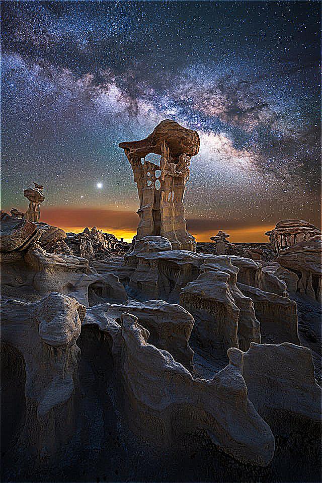
Milky Way Alpha=0.4:
Milky Way Alpha=1:

Milky Way Alpha=5:
Milky Way Alpha=10:
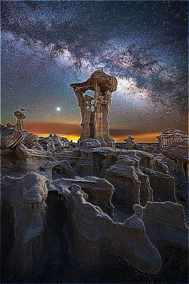
Milky Way Alpha=50:
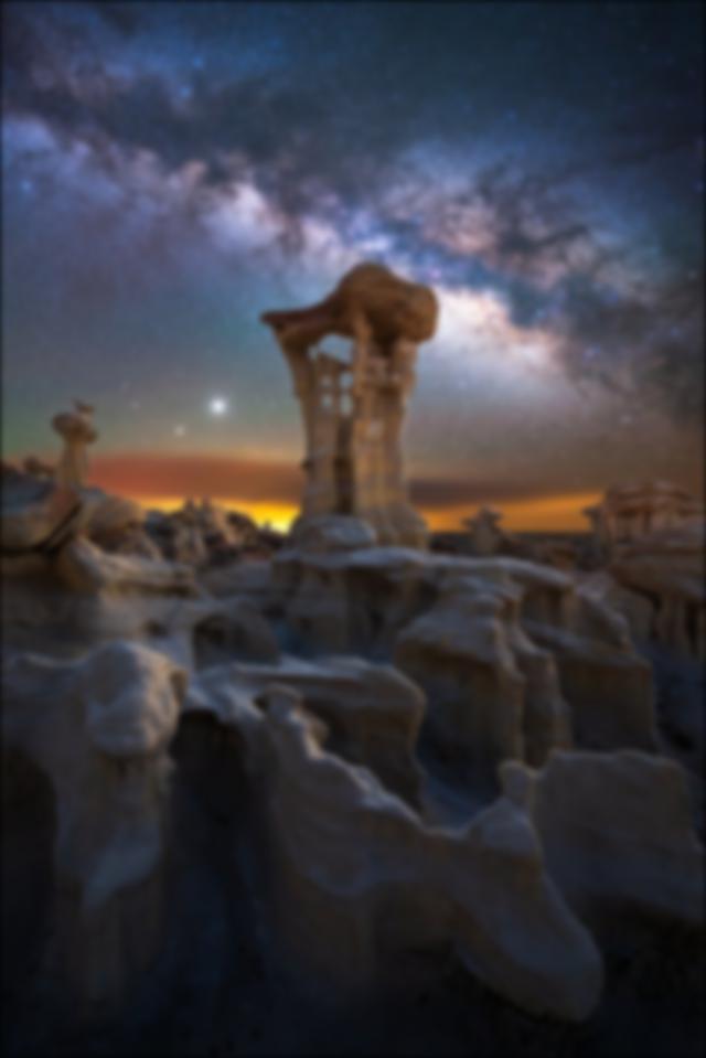
Moreover, we also start with a blurry version of the Milky Way and try to sharpen it.
Milky Way Blurry:

Milky Way Blurry Sharpened Alpha=0.4:
Milky Way Blurry Sharpened Alpha=1:

Milky Way Blurry Sharpened Alpha=5:

Milky Way Blurry Sharpened Alpha=10:

Milky Way Blurry Sharpened Alpha=50:
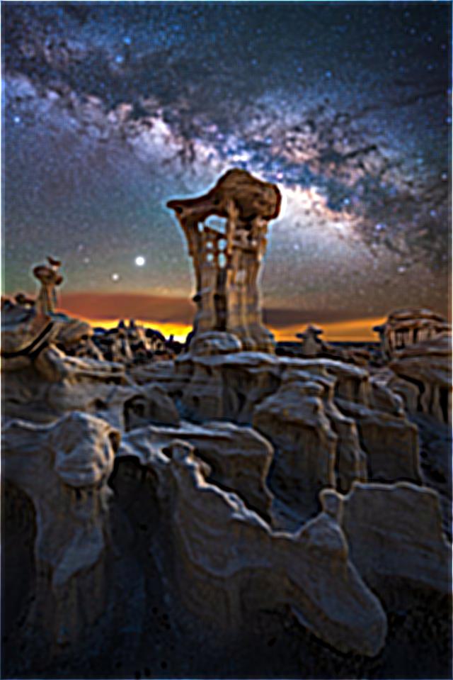
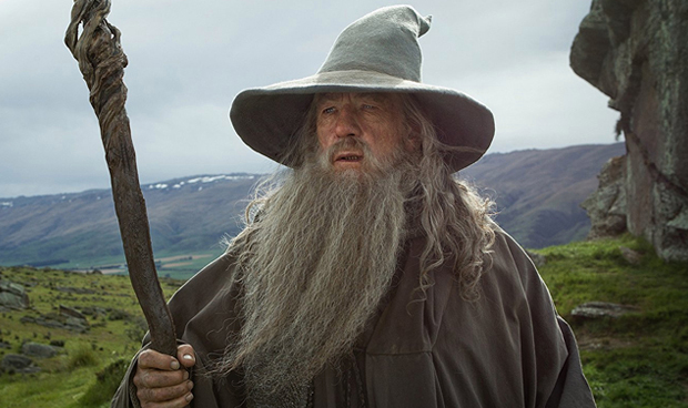
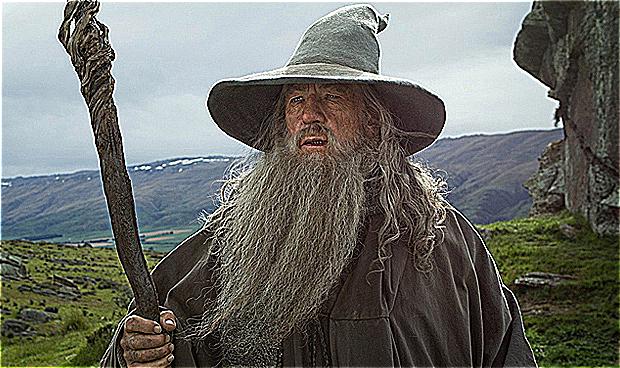
As we can see, the unsharp masking technique only amplifies high frequencies if it exists in the image already. No matter how much we increase the alpha of the blurred image, it does not recover the original image. Since the original image was blurred using a low pass filter, high frequencies don't exist in the image. We see that only when alpha=50, minute high frequencies are amplified. Finally, we have an image of Gandalf to see how the unsharp masking technique behaves with faces.
Gandalf Original:
Gandalf Sharpened Alpha=0.4:

Gandalf Sharpened Alpha=1:

Gandalf Sharpened Alpha=5:
Gandalf Sharpened Alpha=10:
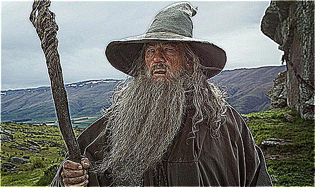
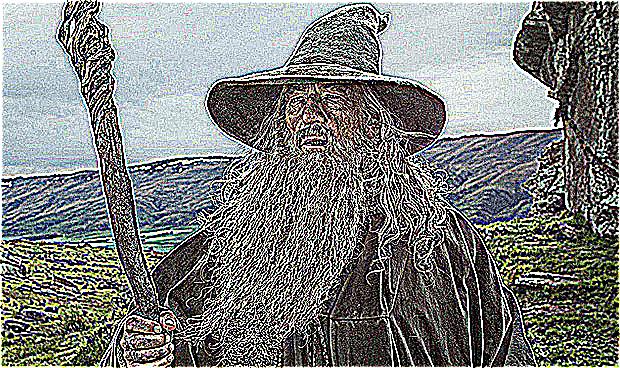
Gandalf Sharpened Alpha=50:
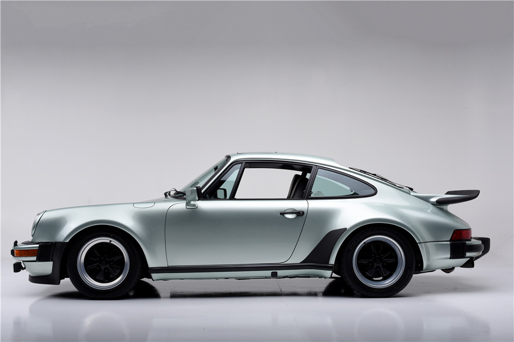
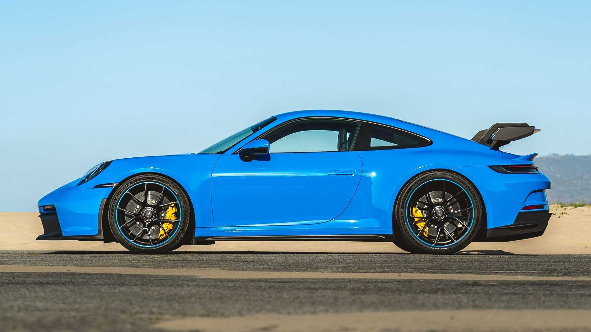
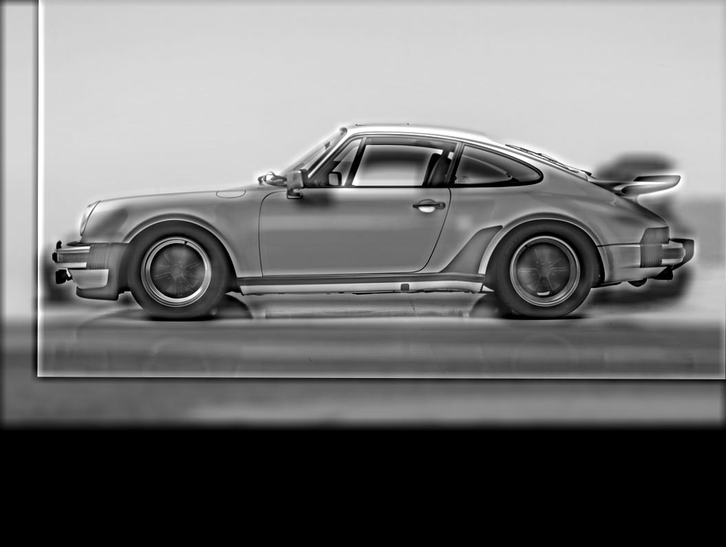
In this implementation, I extract the high frequencies of image 1 and the low frequencies of image 2, summing them together to produce a hybrid image. First my first result, I took an image of a 1977 Porsche 911 and a 2021 Porsche 911. I thought it would be interesting to see them overlaid on each other.
1977 Porsche:
2021 Porsche:
Combined Image:
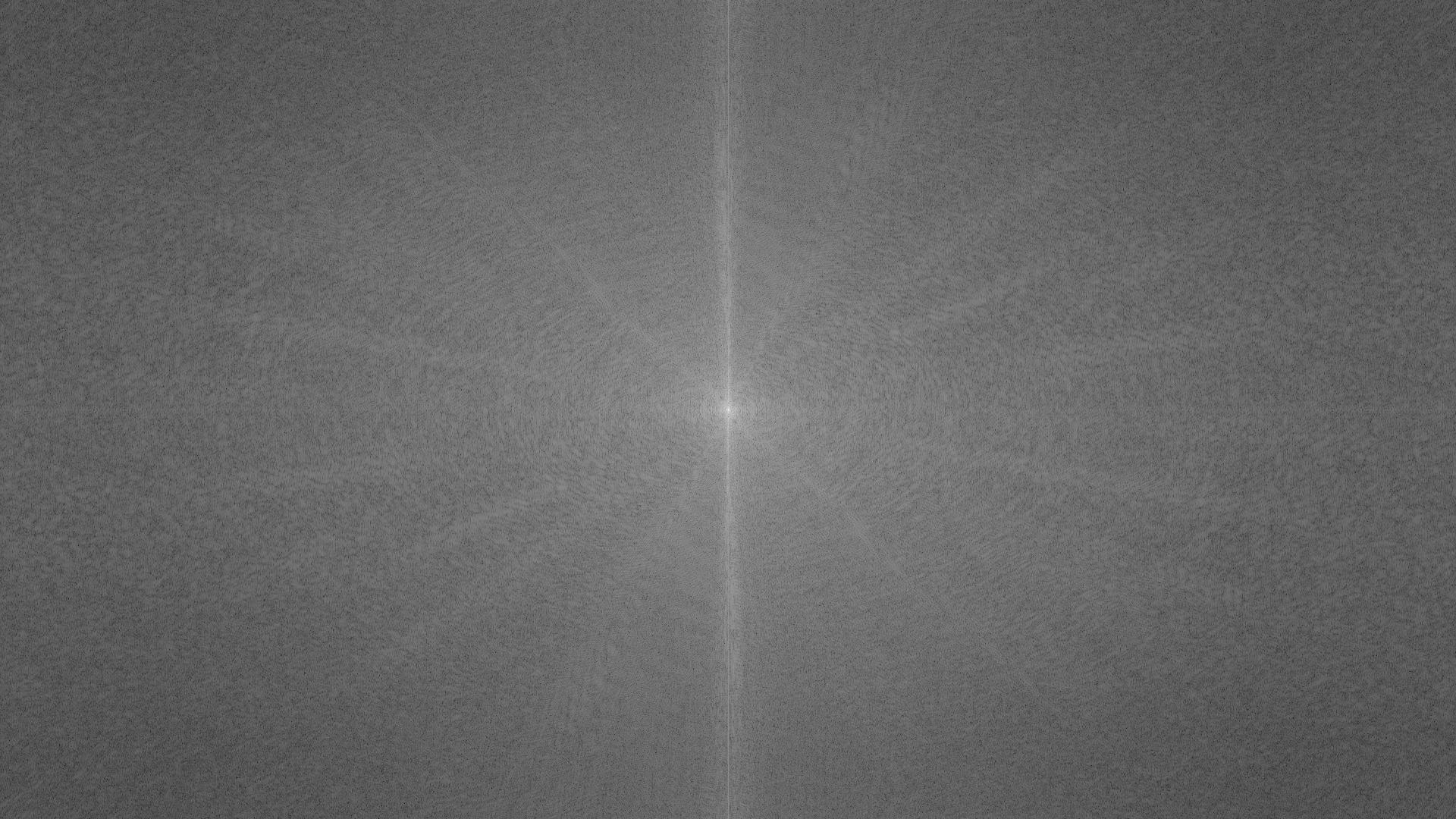
1977 Original Frequency Diagram:
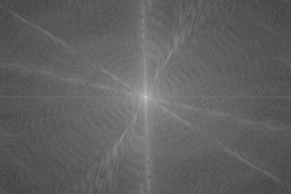
1977 High Frequencies:
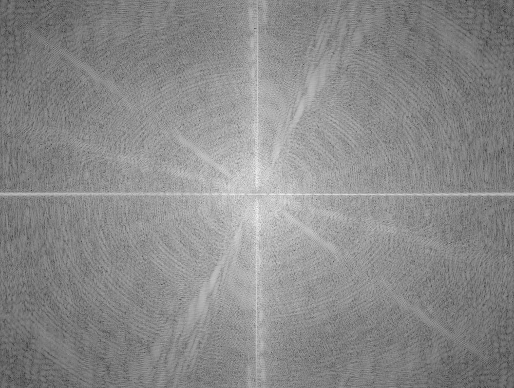
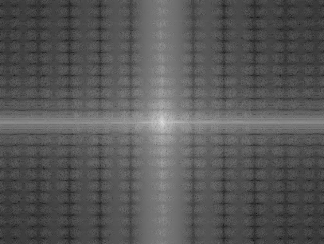
2021 Original Frequencies:
2021 Low Frequencies:
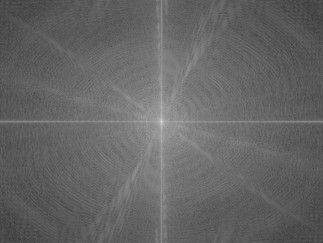
Hybrid Image Frequencies:
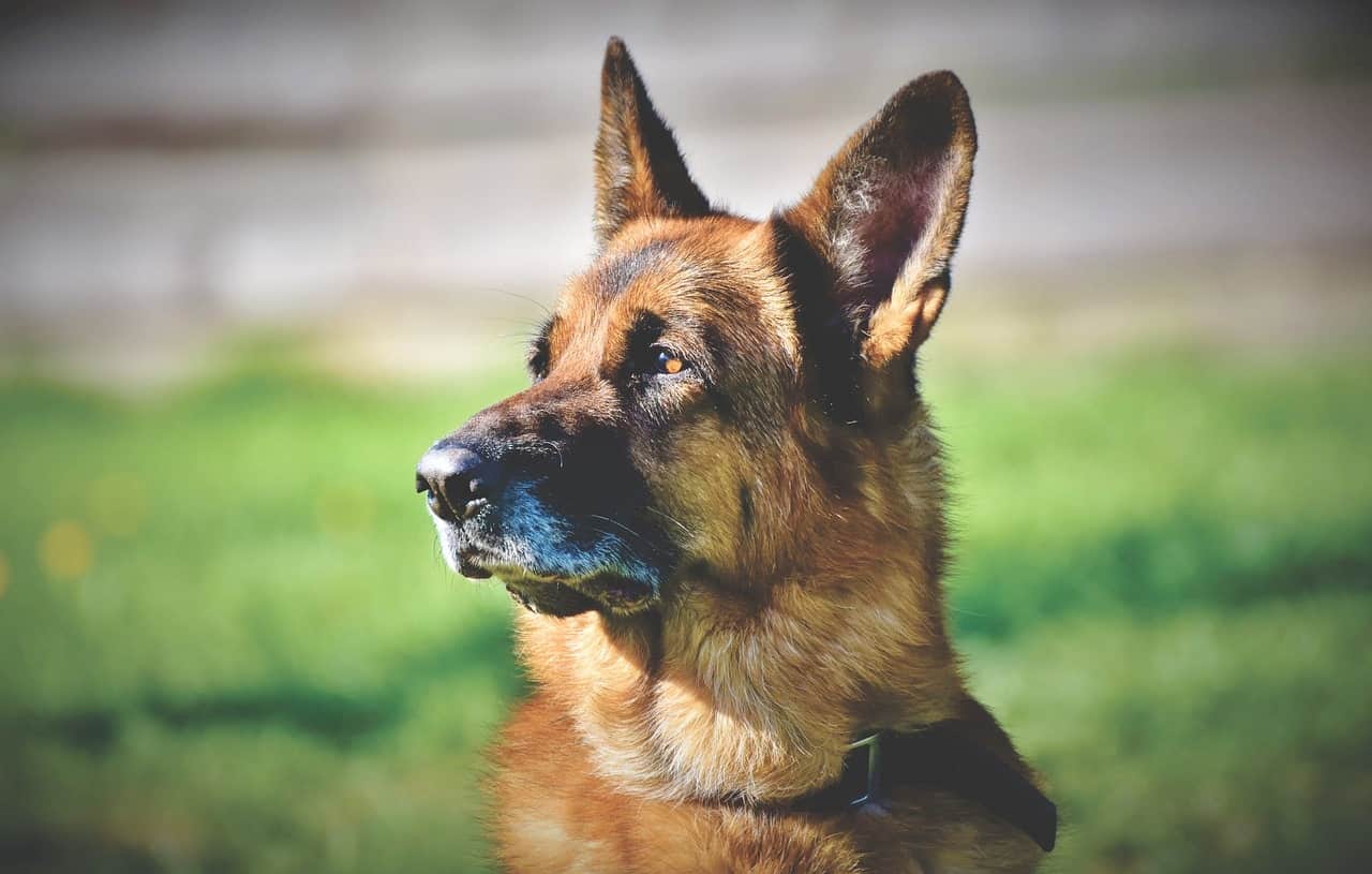
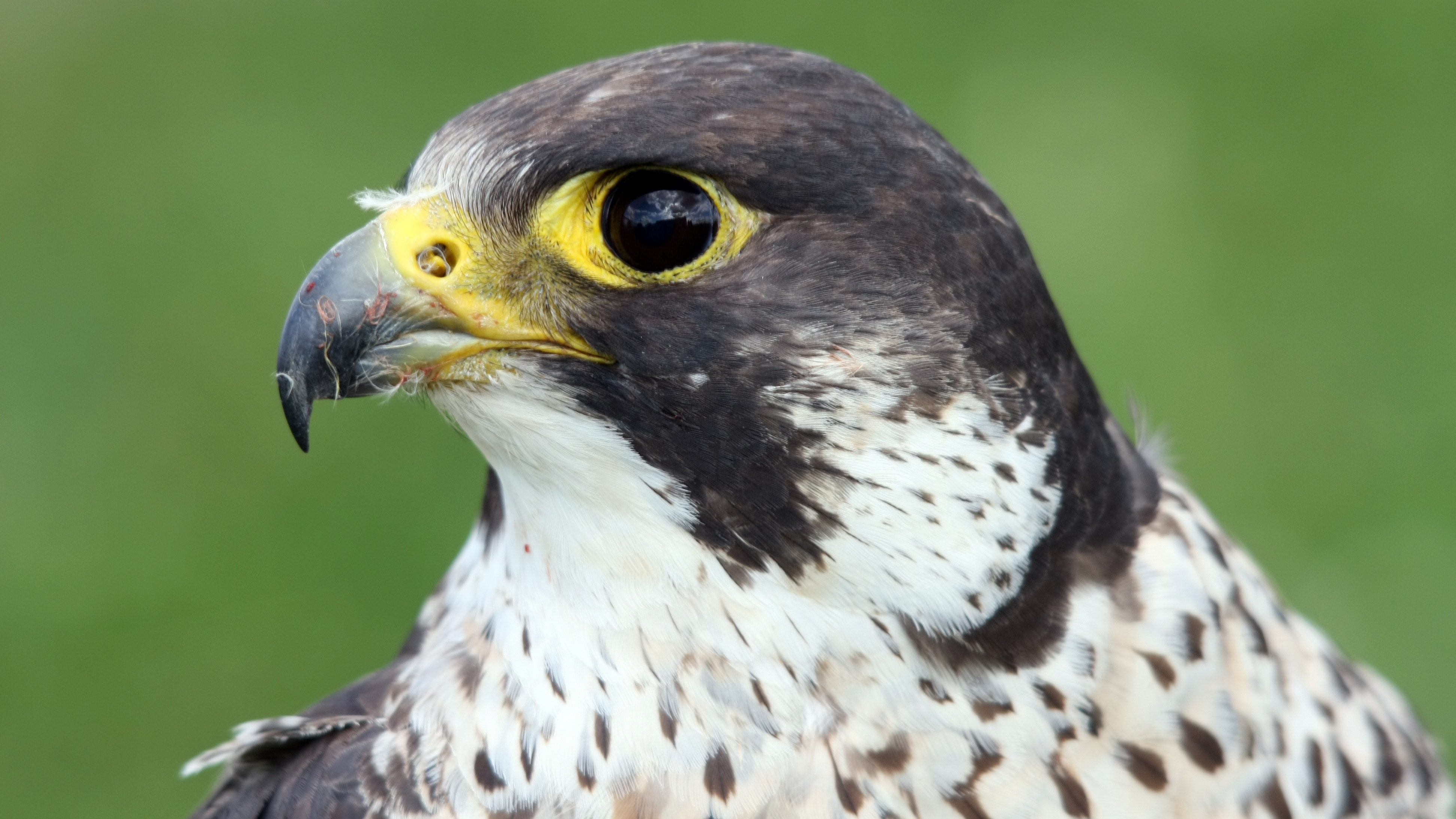
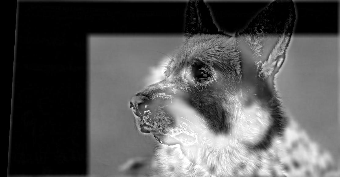
The next example is a dog and falcon.
Original Dog:
Original Falcon:
Hybrid Dog Falcon:
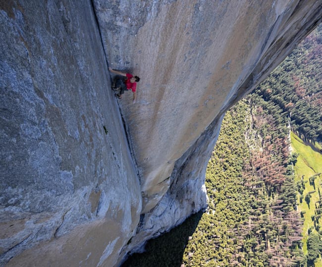
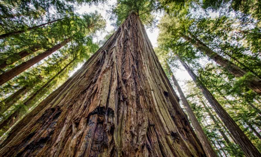
The final example is an image of Alex Honnold (a famous climber) and a Sequoia tree.
Original Honnold:
Original Sequoia:
Hybrid Honnold Sequoia:
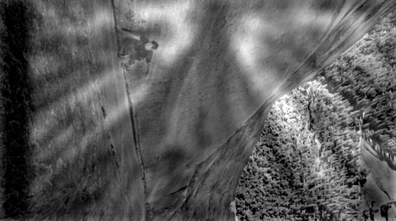
I would consider this example a failure. While it sort of works out, the tree looks more like a shadow, even from a distance. I believe that the reason this failed is because there was no good alignment. I tried to align the rock wall with the tree, but no matter the configuration, it isn't possible to align the two images together well.
In this and the next section, the goal is to combine two images together without a clear seam.
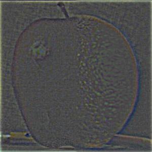
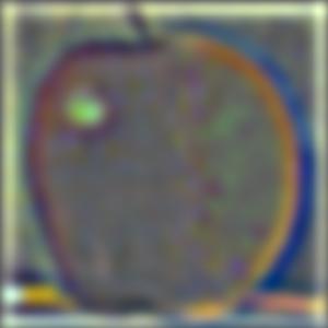
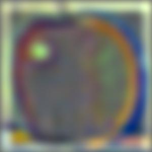
Here is the laplacian stack for the half apple:
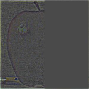
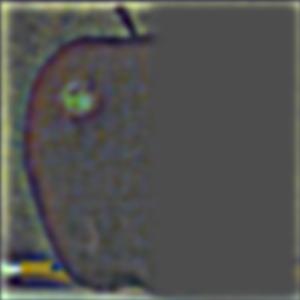
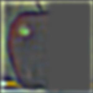
And for the half orange:
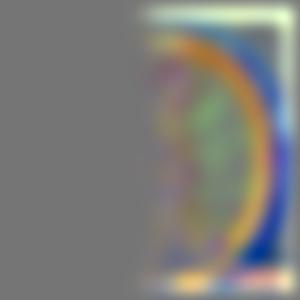
And for the combined image laplacian stack:

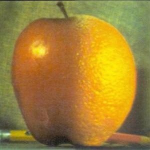
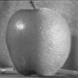
Bells and Whistles - The above images are in color which is the bells and whistles portion for part 2.3 and part 2.4. To demonstrate that my grayscale version also works, I've included the oraple in grayscale.
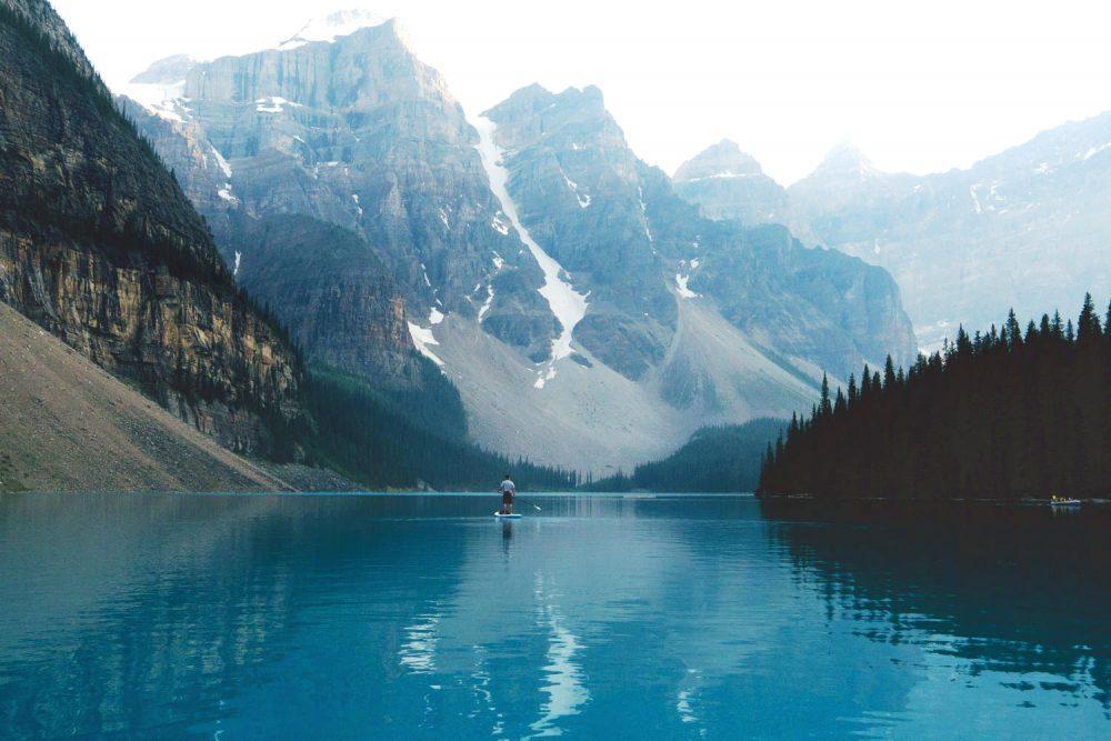
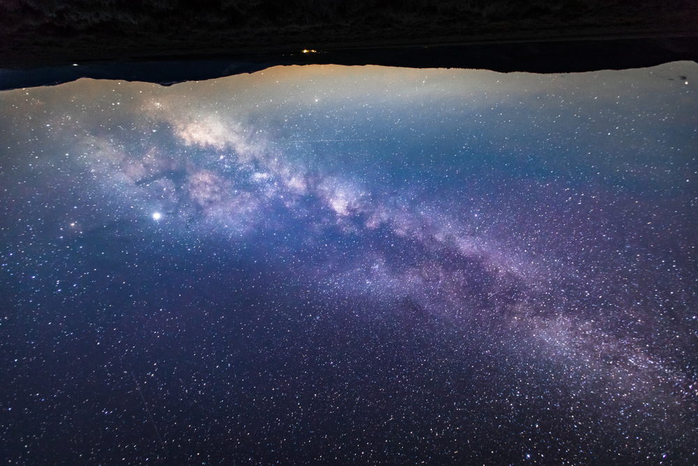
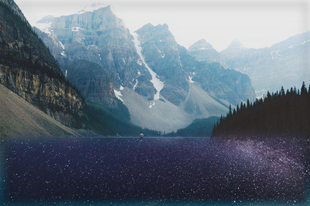
I used the techniques from part 2.3 to develop the next two images. The first one is a combination of the stars and a man kayaking in a lake. The stars image is upside down. The goal is that the man kayaking is riding the stars.
Man Kayaking:
Stars:
Final Combined Image:
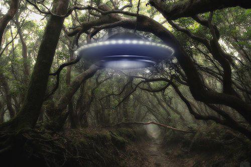
The next example is a combination of a UFO and a jungle. This one uses an irregular mask that I created in photoshop.
UFO Original:
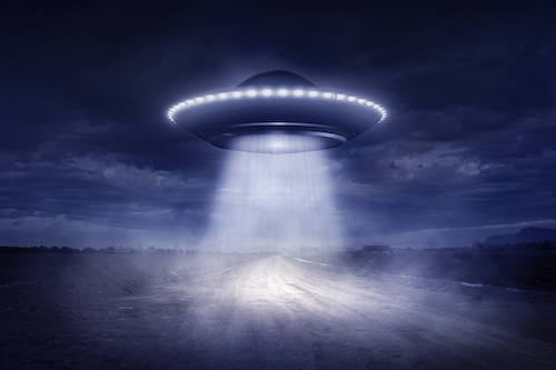
Jungle Original:
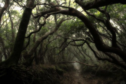
Mask (white=1 and black=0):
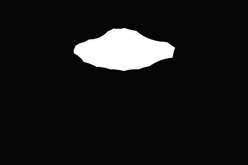
Blended Image: