Overview

Give a high-level overview of what you implemented in this project. Think about what you've built as a whole. Share your thoughts on what interesting things you've learned from completing the project.

Part 1: Fun with Filters

In this part, we will build intuitions about 2D convolutions and filtering.

Part 1.1: Finite Difference Operator

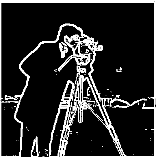
In this part, we are given an image of a camera man. We begin by using the Dx = [1, -1], Dy = [[1], [-1]] to to convolve with the original image in order to find the partial derivative in x and y. Then we use the equation g=sqrt(px^2+py^2) to find the gradient, where px and py are the pixels from the partial derivatives. Finally, we binarize the gradient magnitude image by picking a threashold(0.15 for my implementation), to suppress the noise while showing all the real edges.

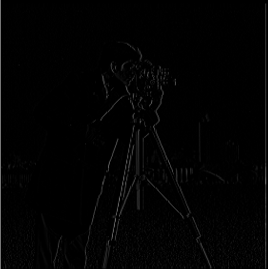
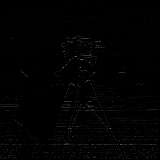
Part 1.2: Derivative of Gaussian (DoG) Filter

We noticed that with the previous steps, the edge image created contains quite some noise. In order to reduce the noise, we can use a smoothing operator to convolve with the original image before we carry out the operations above. In this implementation, we used a 2D gaussian filter(kernel size = 7, sigma = 5) to convolve with the cameraman image.

As we can see from the image below, the amount of noise is greatly reduced. The edge image is much cleaner.

Alternatively, we can do the same thing with a single convolution instead of two by creating a derivative of gaussian(DoG) filters. We can convolve the gaussian filter with Dx and Dy from the previous part before the operations.

It produces the same results as the original DoG method above.

Notice here the shape of DoG filters are different from the original image. This is because when we creat the DoG filters by convolving the gaussian with Dx and Dy, we need to choose the mode to be 'full' instead of 'same' for the operations to work.

Part 2: Fun with Frequencies!

In this part, we will manipulate frequencies of images to create interesting results.

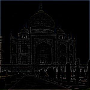
Part 2.1 Image "Sharpening"

In this part, we first use a Gaussian filter(kernel size = 9, sigma = 3) as a low pass filter to retain only the low frequencies. Then we subtract the blurred version from the original image to get the high frequencies of the image. An image is visually sharper if it has stronger high frequencies.

This can also be done in a single convolution by creating a unsharp mask filter, which can be done by using an unit impulse filter, with an arbituray alpha (alpha = 1 im my implementation).

Below are the sharped images created using this methods. I also included some images I chose from the Internet.

If we were to blur an image first then to sharpen it with the unsharp mask, it does not work very well since some information is lost when we low pass the original image with the Gaussian filter.

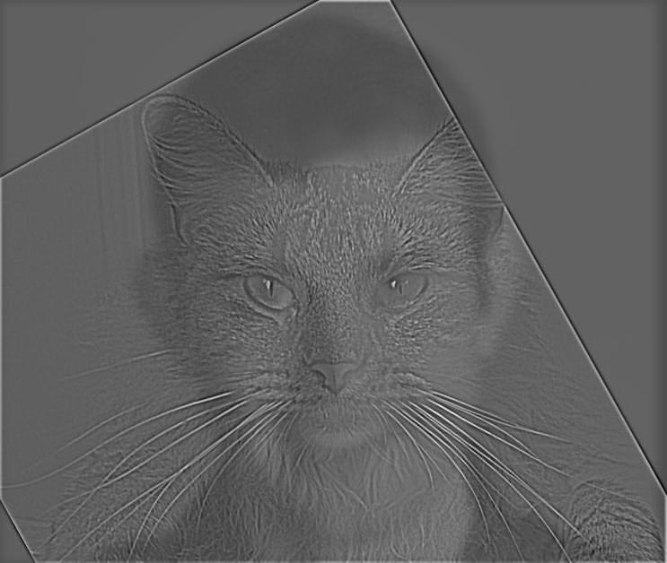
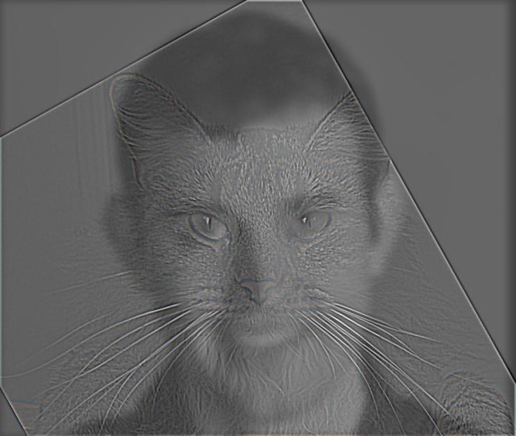
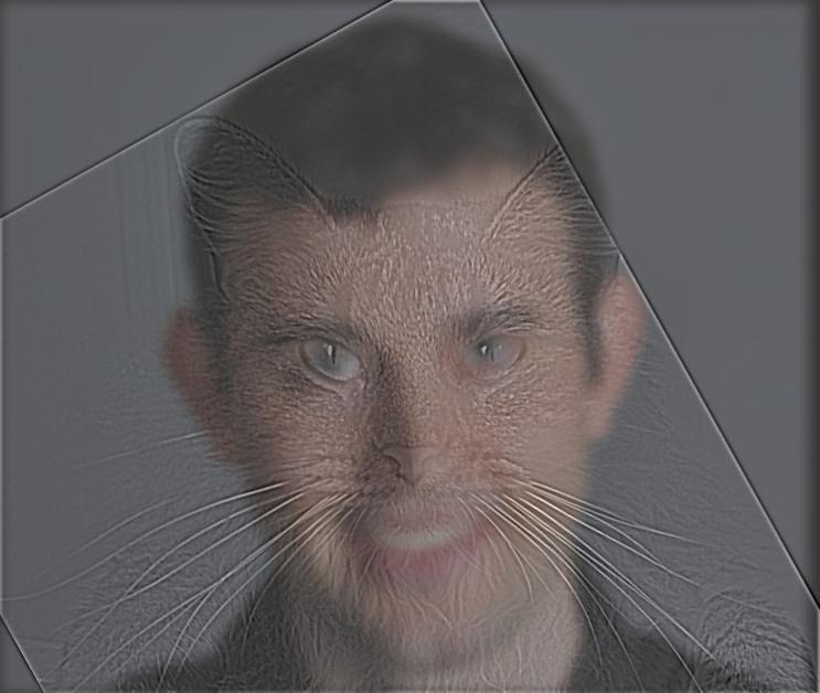
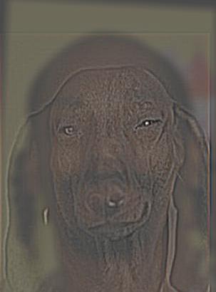
Part 2.2: Hybrid Images

The goal of this part of the assignment is to create hybrid images using the approach described in the SIGGRAPH 2006 paper by Oliva, Torralba, and Schyns. Hybrid images are static images that change in interpretation as a function of the viewing distance. The basic idea is that high frequency tends to dominate perception when it is available, but, at a distance, only the low frequency (smooth) part of the signal can be seen. By blending the high frequency portion of one image with the low-frequency portion of another, you get a hybrid image that leads to different interpretations at different distances.

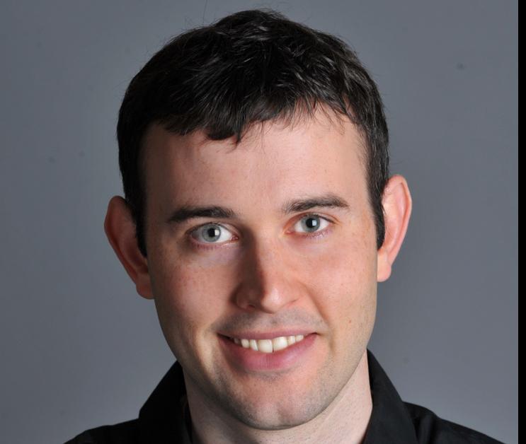
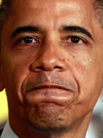
For the first pair of images(Derek and his former cat Nutmeg), we first align two images by mannually picking two reference points. In my implementation, I chose the eyes of Derek and Nutmeg. Then I low passed one image(Derek's) and then high passed the other image(Nutmeg's). Then I added the two images to create a hybrid image.

For a low-pass filter, I used a standard 2D Gaussian filter(ksize=20, sigma=7). For a high-pass filter, I get the result image from subtracting the Gaussian-filtered image(ksize=7, sigma=7) from the original).

Below images were cropped for better viewing experience:

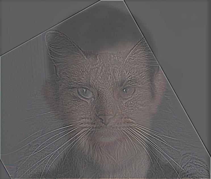
I also tried using color to enhance the effect. I tried three ways: using color for the high-frequency component, using color for the low frequency component, and using color for both components. The results are displayed below:

As seen above, keeping color only for the high frequency component seems to have little effect as compared to grayscale. Using color only for the low frequency makes viewer more likely to recognize the image as a person. This is a reasonable result since color is an important element in visual recognition for human. Hence, among the three, keeping color for both components better achieve the purpose of a blended image, without biasing against any one of the images. Also, I believe that having color is generally better than grayscale, at least from the aesthetic perspective. It gives the viewer more elements to recognize what is in the image.

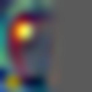
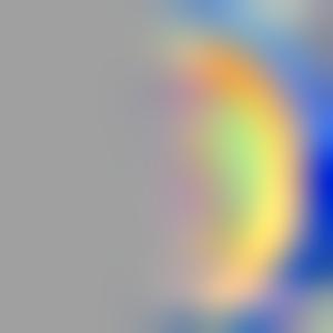
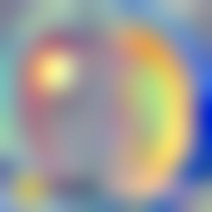
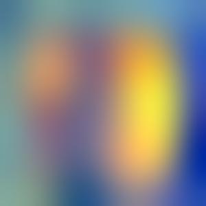
The log magnitude of the Fourier transform of the above hybrid image that keeps color from both components is shown below. It is clear that the high frequencies of Nutmeg's image is added to the low frequencies of Derek's image.

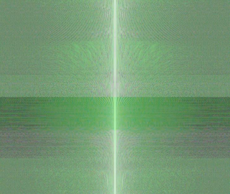
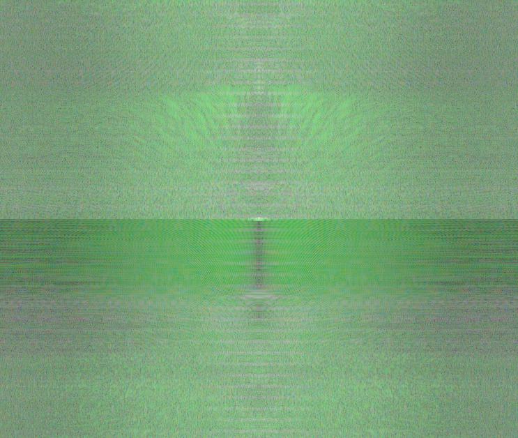
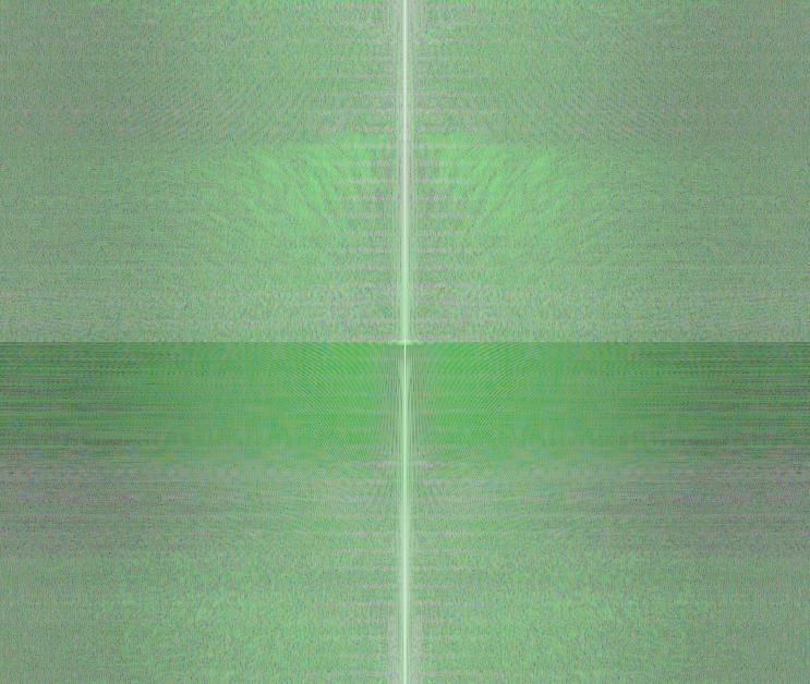
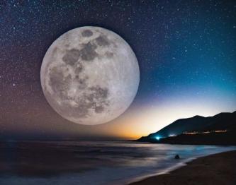
Here are some images I created:

Multi-resolution Blending and the Oraple journey

Part 2.3: Gaussian and Laplacian Stacks

This part aims to to blend two images seamlessly using a multi resolution blending as described in the 1983 paper by Burt and Adelson. An image spline is a smooth seam joining two image together by gently distorting them. Multiresolution blending computes a gentle seam between the two images seperately at each band of image frequencies, resulting in a much smoother seam.

I implemented a Gaussian and a Laplacian stack. The different between a stack and a pyramid is that in each level of the pyramid the image is downsampled, so that the result gets smaller and smaller. In a stack the images are never downsampled so the results are all the same dimension as the original image, and can all be saved in one 3D matrix (if the original image was a grayscale image). To create the successive levels of the Gaussian Stack, just apply the Gaussian filter at each level, but do not subsample. In this way we will get a stack that behaves similarly to a pyramid that was downsampled to half its size at each level.

At each level, I created a Gaussian filter. I convolve this Gaussian filter with the GR mask and the two input images. Then I used the difference between successive levels of the Gaussian stack to create the Laplacian stack. At each level, I applied the GR mask at the level to the two input images at the same level to generate the combined image. Notably, the last level of the Laplacian stack is taken from the last level of the Gaussian stack directly. Since there is no more Gaussian stack for us to take the difference.

To get a more gentle seam, I have different sizes and sigmas at each level, and the blurring is stronger at lower frequencies (lower levels). The sizes and sigmas I used are:

sigmas = [10, 20, 30, 35, 40], sizes = [40, 60, 80, 100, 120].

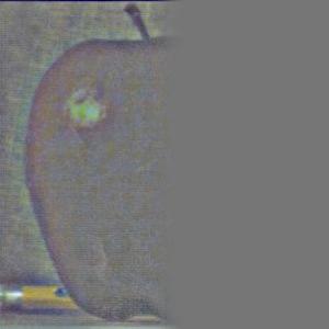
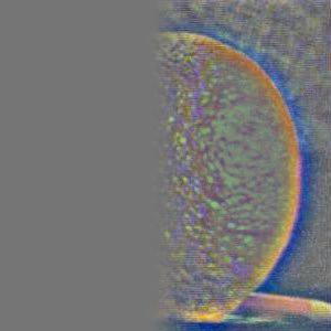
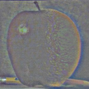
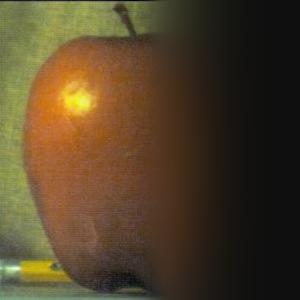
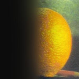
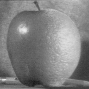
Below are the Laplacian stack blending details of an apple and an orange. The first three rows show the high, medium, and low-frequency parts of the Laplacian stack(taken from levels 0, 2, and 4). The left and middle columns show the original apple and orange images weighted by the smooth interpolation functions, while the right column shows the average contribution.

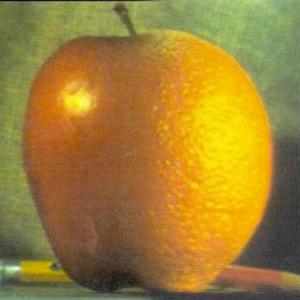
Part 2.4 Multiresolution Blending (a.k.a. the oraple!)

In this part, I used the Gaussian and Laplacian stack I created in the previous part to blend together the apple and the orange to an orple. This can be done by collapsing the Laplacian stack generated from the apple and the orange input images. I have also created a colored blend below.

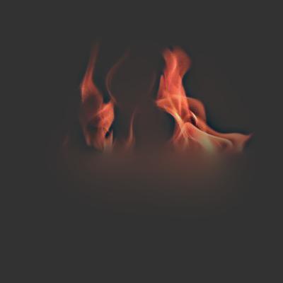
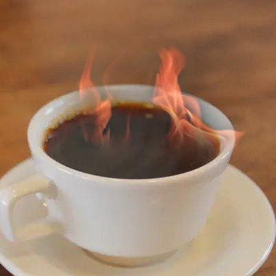
Here are two images I blended together:

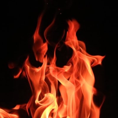
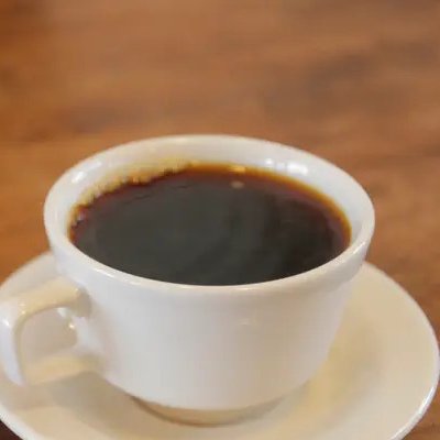
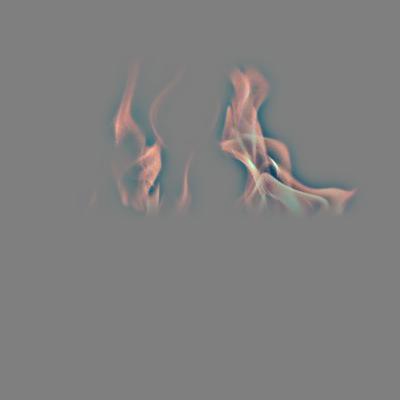
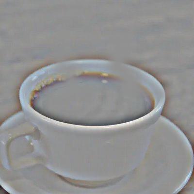
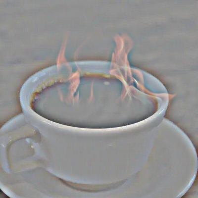
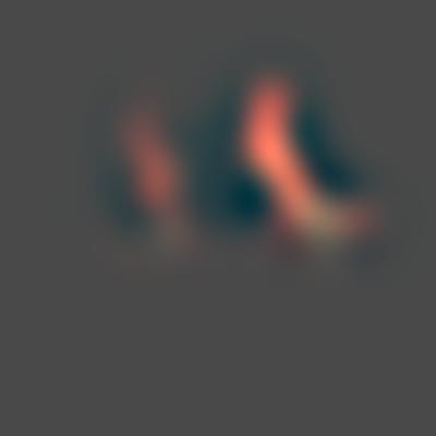
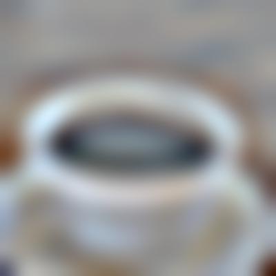
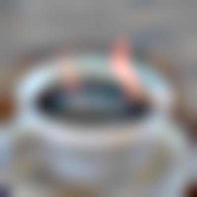
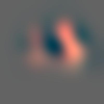
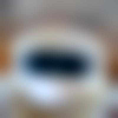
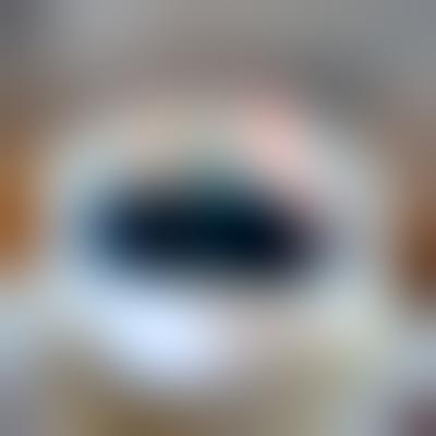
Similar to Part 2.3, I created the intermediate Laplacian results of the fire coffee below to better visualize the process:

Conclusion

As a photography enthusiast, I used photoshop/lightroom a lot. The coolest part of the project for me is that I did something I thought I could only do in the editing tools, now with code. It definitely helps me understand some of the workings behind those image editing tools. This is really cool and interesting!

Reference

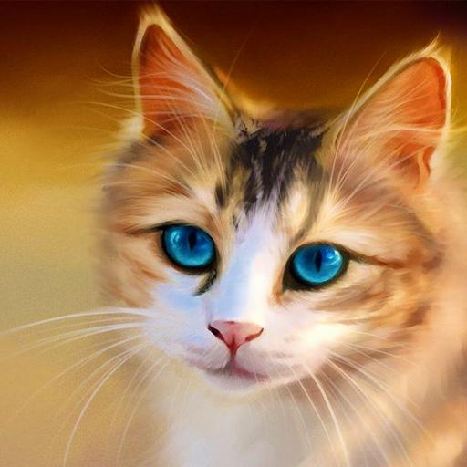
Kitty https://www.amazon.com/Cat-Wallpaper-Cute-Cats-Kittens/dp/B08KJD6C2L

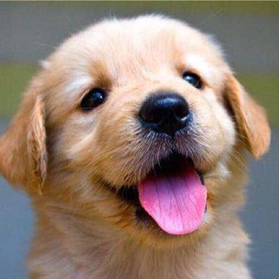
Puppy https://www.pinterest.com/pin/693272936362405474/

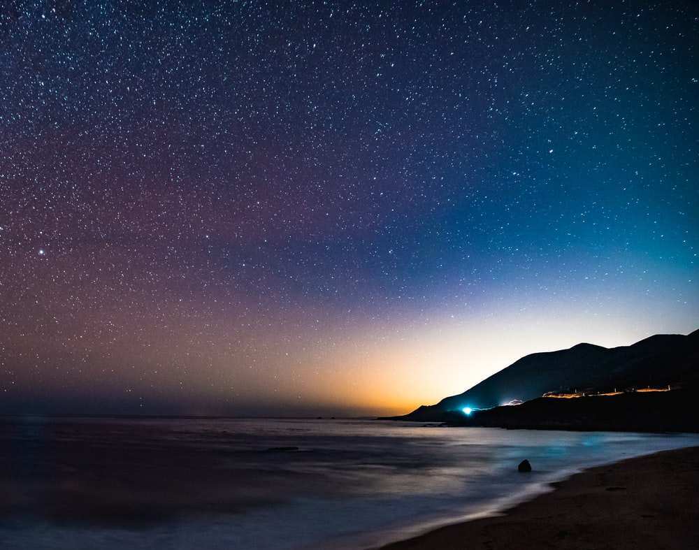
Beach https://www.google.com/imgres?imgurl=http://www.xgcs123.com/p/1288aqwr/0149.jpg&imgrefurl=https://asujenggong-jp.web.app/fucebe-%25E5%25A3%2581%25E7%25B4%2599-%25E9%25A2%25A8%25E6%2599%25AF.html&h=348&w=620&tbnid=3N67NQQvwISiQM&tbnh=168&tbnw=300&usg=AI4_-kQ1rYseDnIXMW7JBIWtPwJgxANw1w&vet=1&docid=5rt8qHVM9HcaKM&itg=1&hl=zh_CN#imgrc=3N67NQQvwISiQM&imgdii=rboYDVWQuftY3M

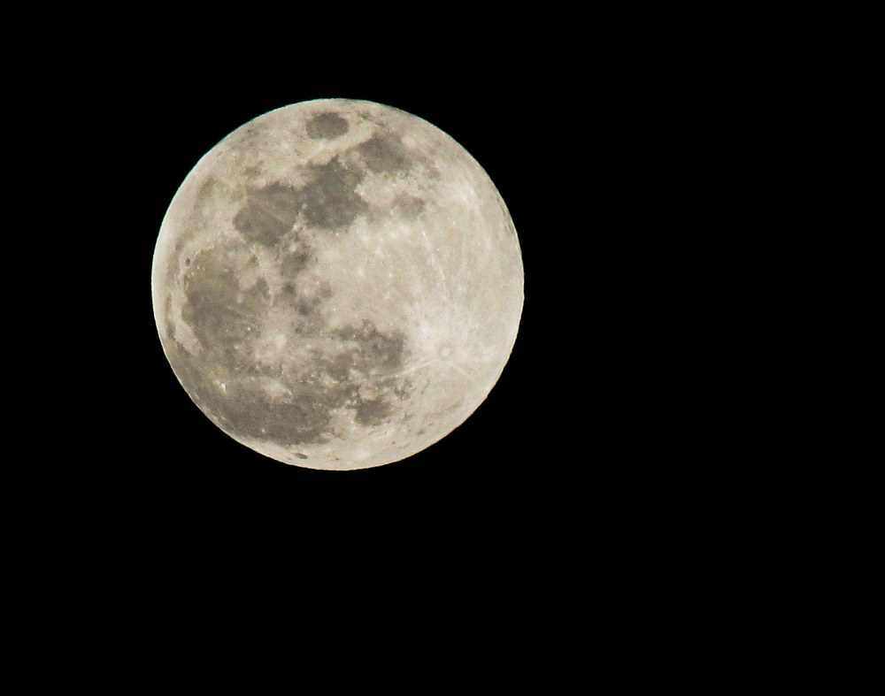
Moon https://www.flickr.com/photos/mzmo/3186645474

Fire https://unsplash.com/s/photos/fire

Coffee https://www.insider.com/drinking-4-cups-of-coffee-a-day-strengthens-your-liver-2021-6