Fun with Filters and Frequencies!

Kyle Hua, CS194-26-AGX

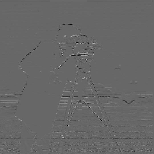
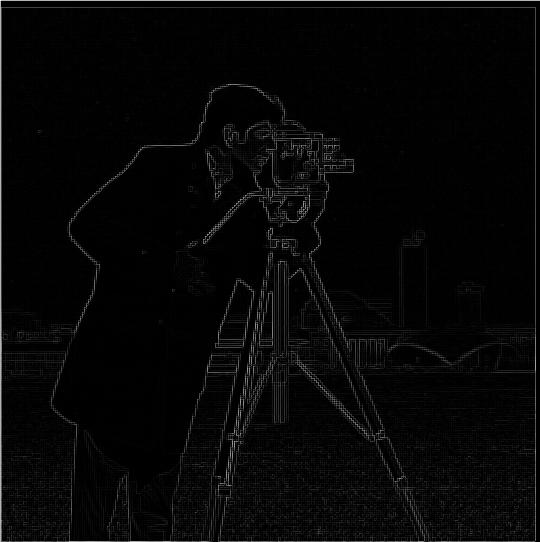
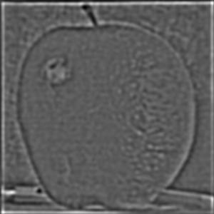
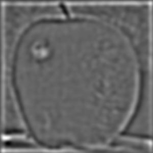
1.1 Finite Difference Operator

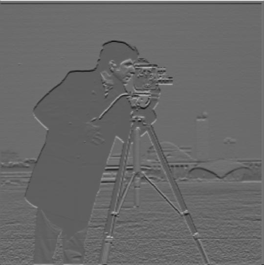
Using the finite difference operators dx and dy, we can convolve the operators with an image to get the partial derivatives of the image. From the partial derivatives, we can compute the gradient magnitude image by using the Pythagorean Theorem. To further highlight the edges in the gradient magnitude, we can binarize the image through a threshold.

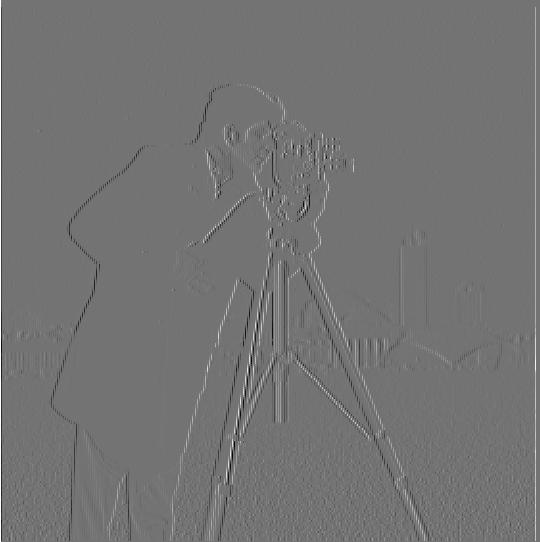
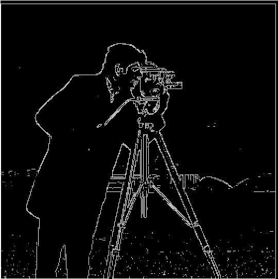
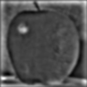
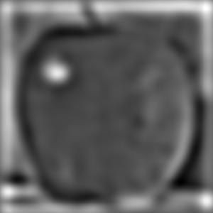
1.2 Derivative of Gaussian (DoG) Filter

The above results are noisey and not super fine grain. To improve on it, convolving the image with the Gaussian filter to blur it beforehand can filter out some of the higher frequency noise leaving us with smoother edges. Running the same procedure will result in the binarized edge image being much more accurate and clean.

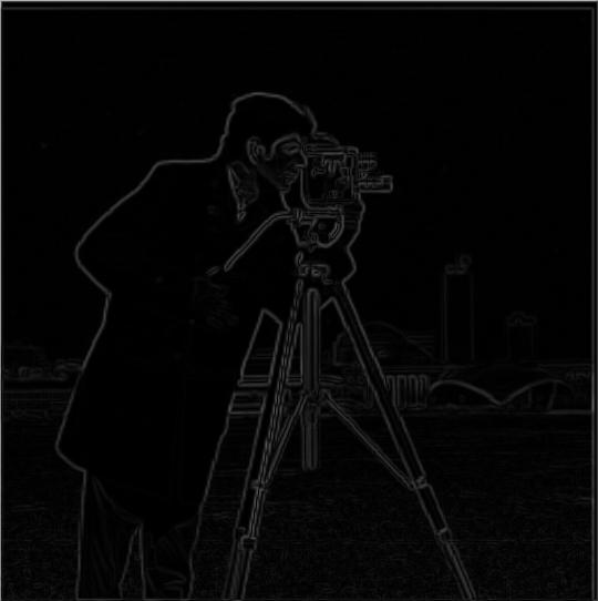
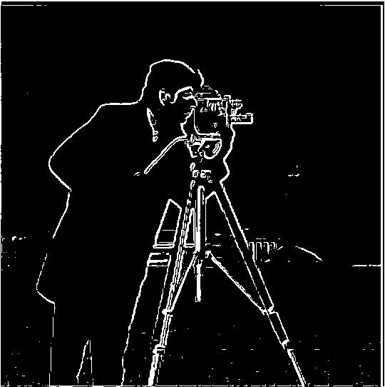
The images clearly show finer edges and more details.

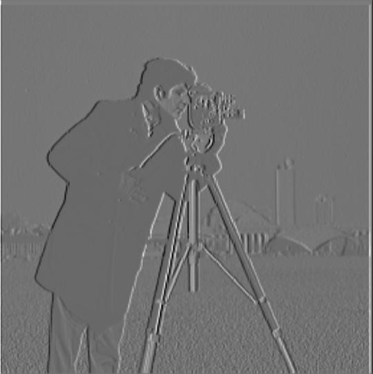
2.1: Image "Sharpening"

To sharpen an image, we need to highlight higher frequencies in the image. Taking the difference between the original image and the image filtered using a Gaussian, yields an the higher frequencies. Adding the higher ones back into the original "sharpens" the image. We can multiply the frequencies by an alpha value to increase the effect.

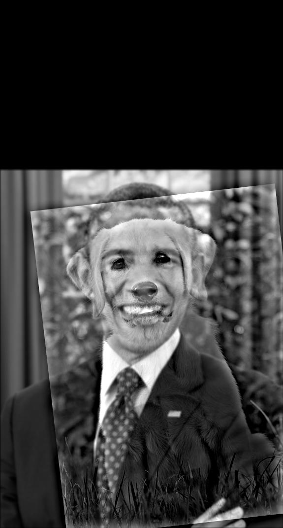
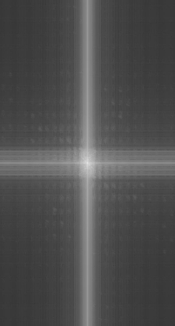
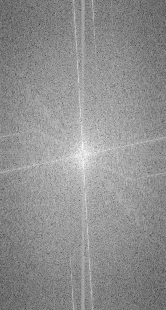
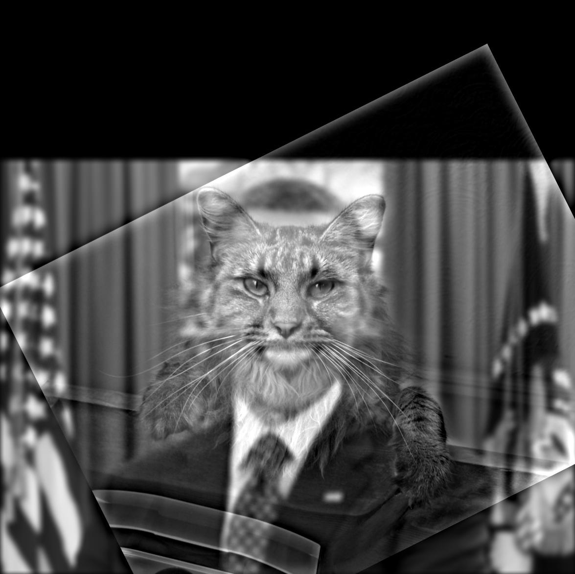
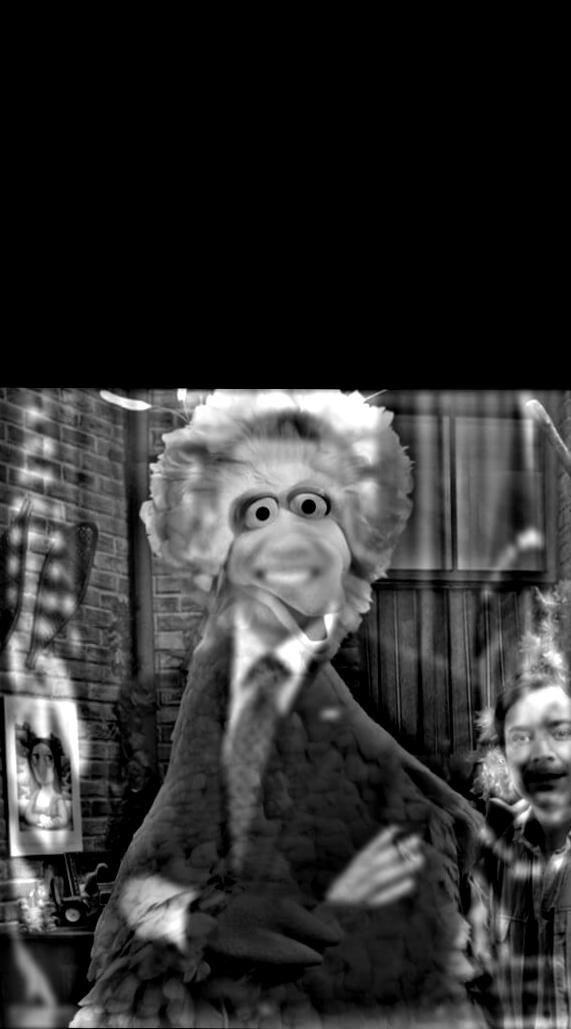
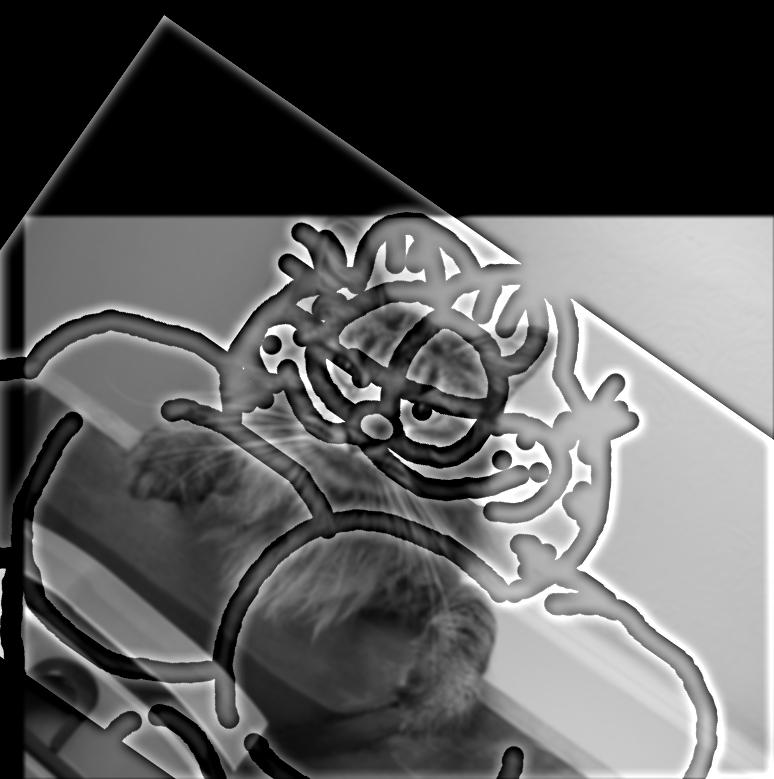
2.2: Hybrid Images

To create hybrid images we combine the high frequency parts of one image with the low frequncy parts of another. Filtering the first image with a Gaussian filter gives us the low-frequency portion of the first image. The high-frequency part of the second image, requires us to take the difference between the second image and the second image filtered with a Gaussia filter.

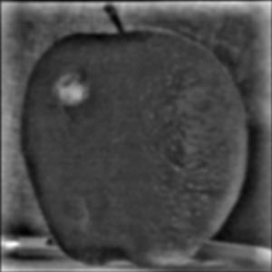
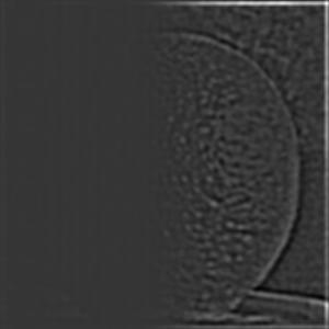
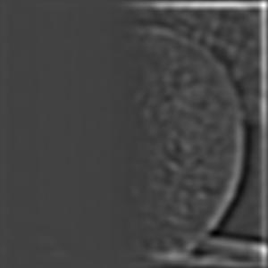
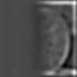
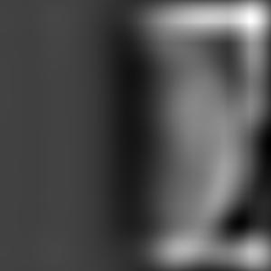
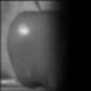
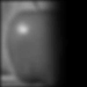
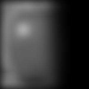
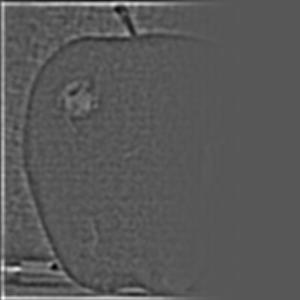
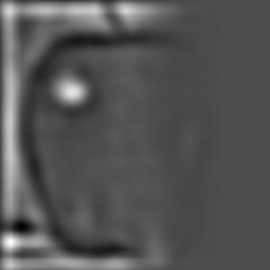
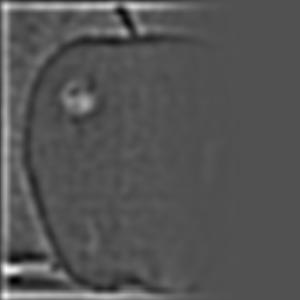
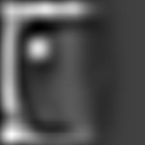
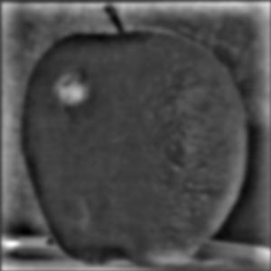
2.3: Gaussian and Laplacian Stacks

We implemented Gaussian and Laplacian stacks. The same image is convolved with a Gaussian filter of increasing sigma (doubling) at each level. Every level is the same size, but higher levels are coarser. We get the Laplacian stack by taking the difference between the image from the Gaussian stack of the same level and the image from the Gaussian stack of the next level.

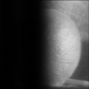
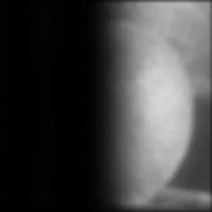
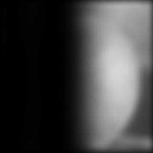
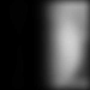
Orange Gaussian and Laplacian

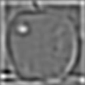
Apple Gaussian and Laplacian

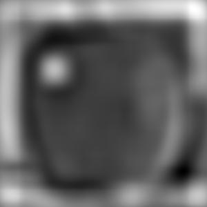
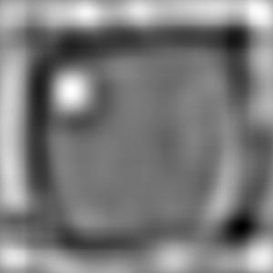
Combined Gaussian and Laplacian

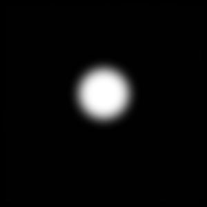
Mask Gaussian (is a mask of the last combined image)

2.4: Multiresolution Blending

To blend an image along a spine we need to: creating an image mask, taking its Gaussian stack; take the Laplacian stack of image 1 and image 2; and then, at each level of the stacks, compute the combined image as per the equation below. LA being Laplacian of image 1 and LB being Laplacian of image 2. Summing the the combine layers yields the combined image.