Original Image
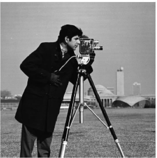
The goal of this project was to experiment with different filtering techniques in order to create cool effects.
Original Image
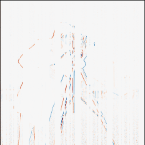
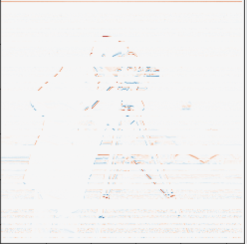
The first step was to use the finite difference operators to get the x and y partial derivatives. They are shown below:
Partial Derivatives in X and Y:
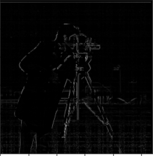
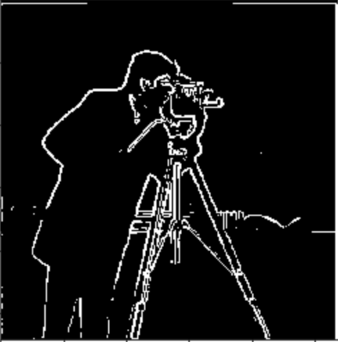
Next, we use the follwing formula to compute a gradient magnitude image: grad = np.sqrt(im_out_dx**2 + im_out_dy**2). Lastly, we binarize the image using a threshold, in this case 0.25.
Grad Magnitude Image and Edge Image

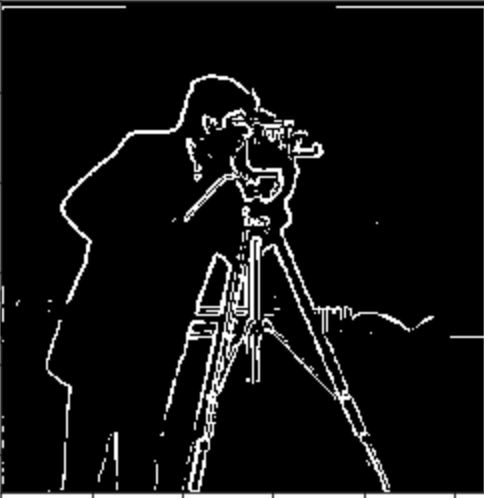
For this part, we experiment with using a gaussian blur to generate an edge image with less noise. By first blurring the image with a gaussian kernel and repearting the process from the last part, we get the results below:
Edge Image After First Applying Gaussian blur
We can see a noticible difference, where the edges appear more crisp and the edge image has less noise than in the previous part.
In order to save a convolution operation we can use a trick! We can convolve the finite difference operator and the gaussian kernel first before convolving with the image. Doing so, we get the same results:
Edge Image After First Applying Gaussian blur, using DoG Filters
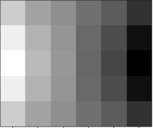
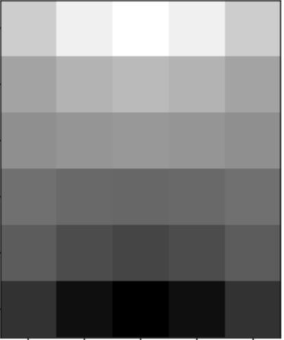
Here are what the DoG Filters look like:
Derivative of Gaussian Filters (left: D_x, right: D_y)
For this part, we use the unsharp mask filter to "sharpen" images. Since the gaussian blur acts as a low pass filter, we can subtract the original image by the blurred image to get just the high frequencies. Then we can add a small amount more of these high frequencies to the original image to get a "sharpened" image. The alpha parameter controls how much of the details we add to the original image. As we increase alpha, we can see that the image appears sharper.
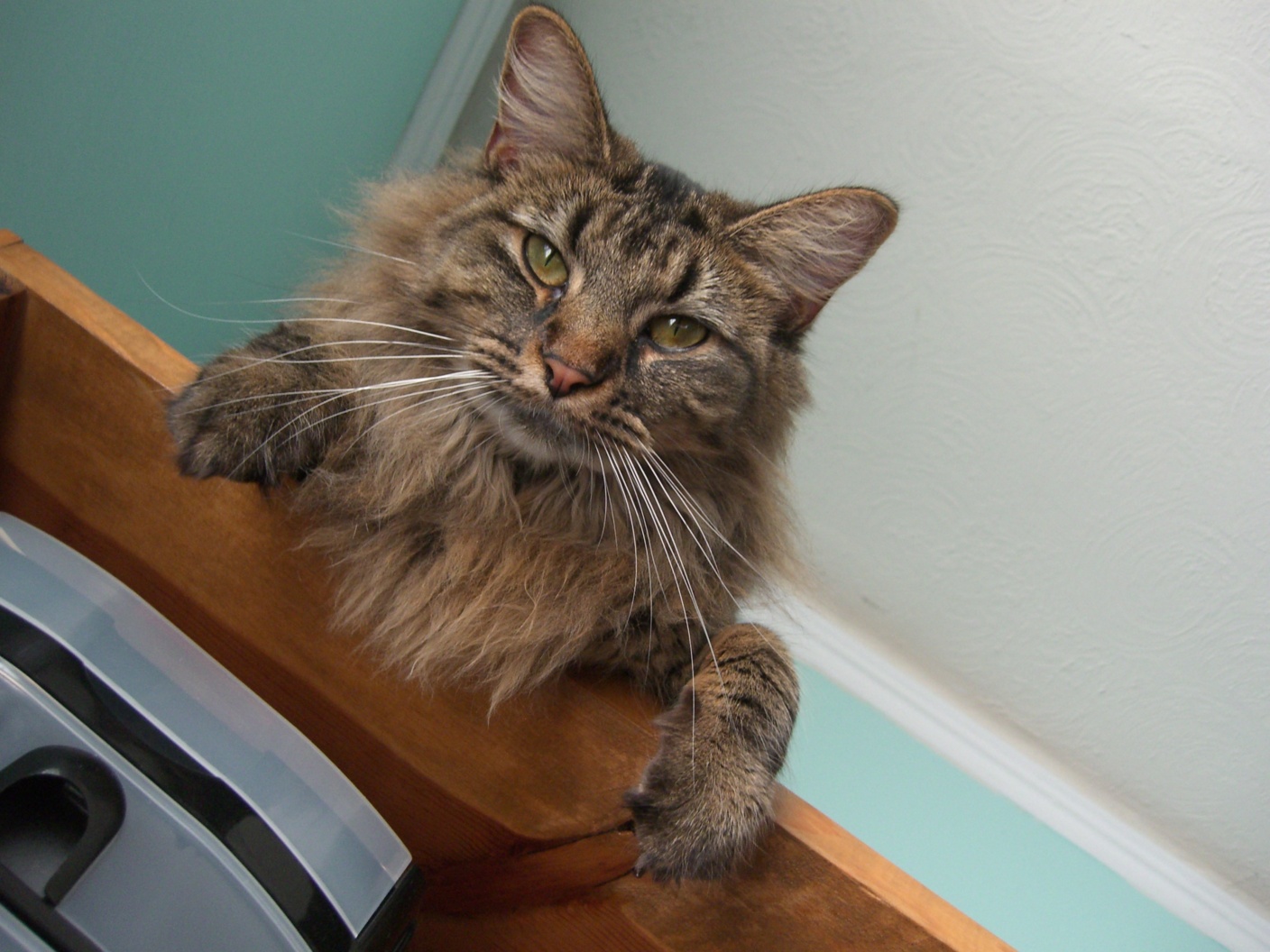
Original Image
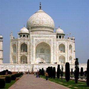
Progression of Sharpening for Taj Mahal (alpha = 0.5, 1, 2, 3)


We will also experiment with taking a sharp image, blurring it, and then resharpening it
Original, already sharp image
Blurred and Resharpened
Although at first glance the images seem the same, the resharpened image is actually worse quality and some of the detail is lost.
Derek and Nutmeg
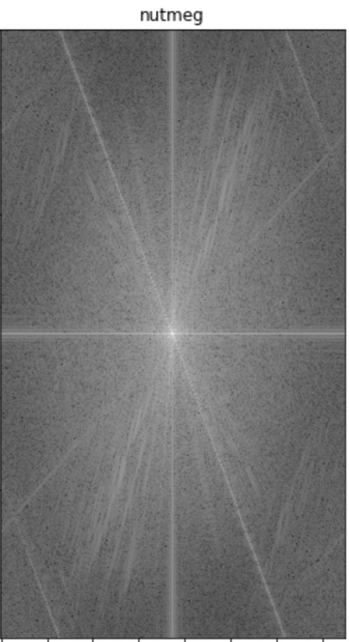
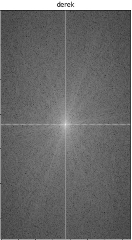
Below is the Fourier analysis of the process:
Log Magnitude of the Fourier transform (Original Derek and Nutmeg)
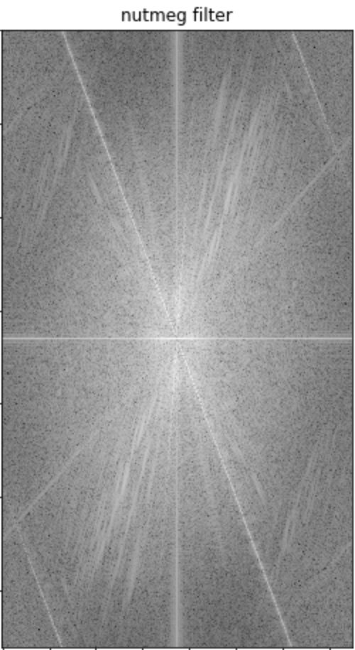
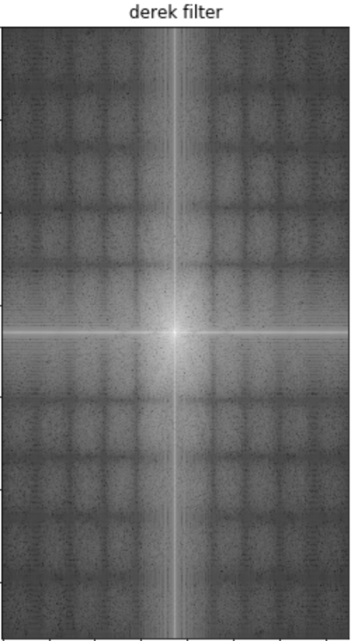
Log Magnitude of the Fourier transform (Filtered Derek and Nutmeg)
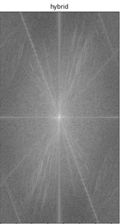
Log Magnitude of the Fourier transform (Hybrid Image)
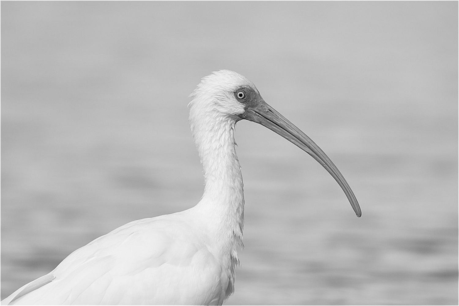
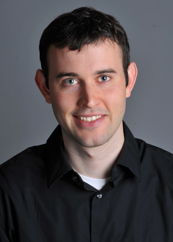
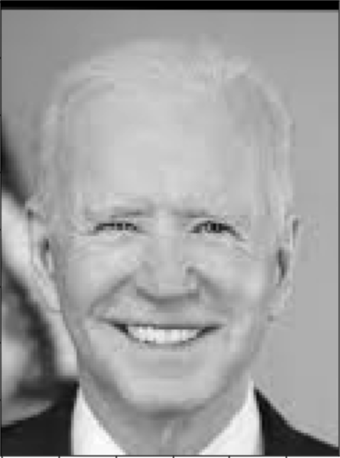
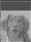
Joe Biden and Dog

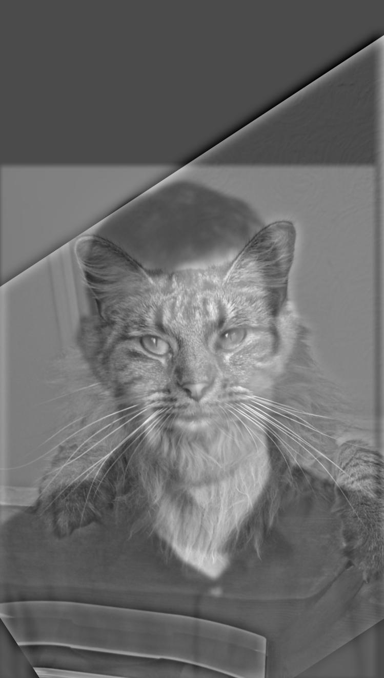
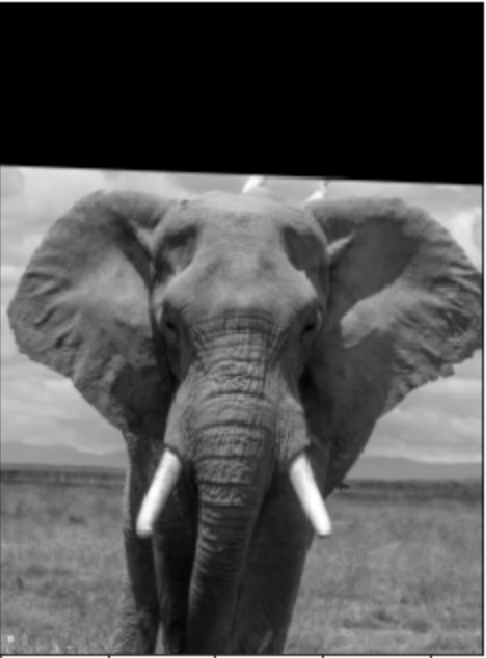
Elephant and Dog (Failed Example)
I tried to create an elephant dog hybrid, but it didn't work as well as the biden dog hybrid. I suspect that this is because the elephant is much larger than the dog which causes problems when trying to separate the frequencies. In addition, the elephant's trunk seems to causing some problems with covering the dog's face.
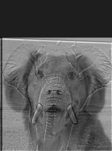
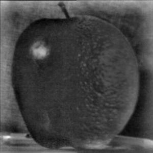
This part involved creating gaussian and laplacian stacks in order to blend 2 images together without leaving a visible seam. First, we will horizontally blend an apple and an orange to create an oraple!
Apple and Orange (Original)
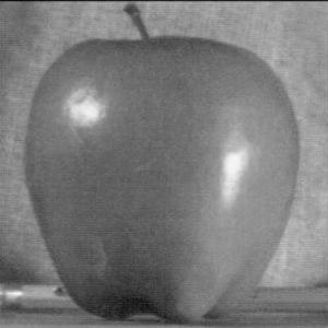
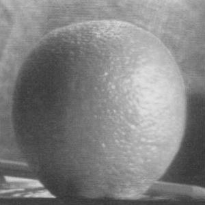
Apple and Orange Laplacian Stack
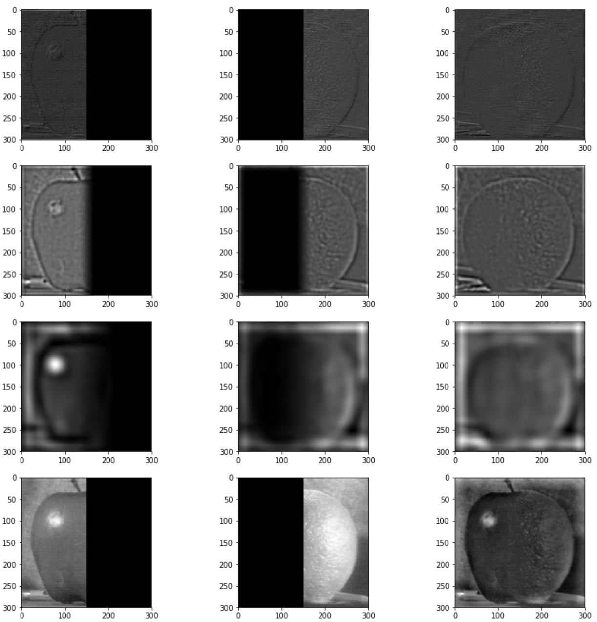
To create our oracle, we first create laplacian stacks of depth 5 for the apple (LA) and the orange (LB). Next, we create a horizontal mask R and create a gaussian stack GR. Next, we create a combined stack using the formula LS = GR * LA + (1 - GR) * LB. We can then sum over all 5 levels to get our final blended image.
Blended Oraple!
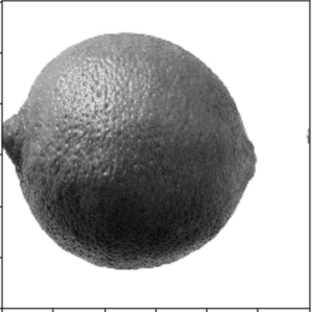
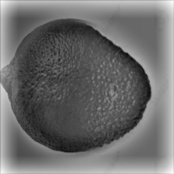
I have repeated the same process to create a lime-avocado hybrid, pictured below. Because the images were taken from Google, I had to manually rescale and shift the images to make the two fruits line up properly.
Limacado

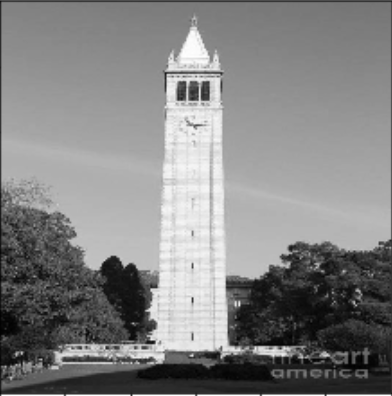
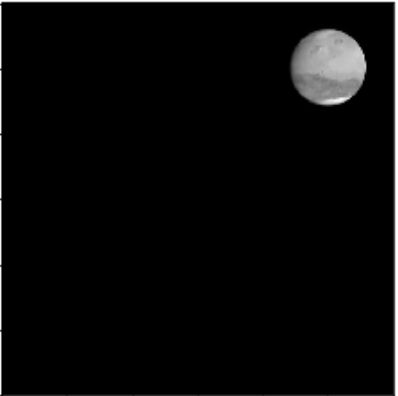
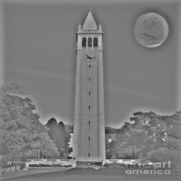
Lastly, I used an irregular, circular mask to blend mars into the sky behind the campanile.
Campanile with Mars
All in all, I learned a lot from this project. The biggest thing I learned was about how different frequencies can be isolated using a Gaussian filter, and how the Gaussian blur acts just like a low pass filter.