Project 2: Abel Yagubyan

Part 1.1 - Finite Difference Operator

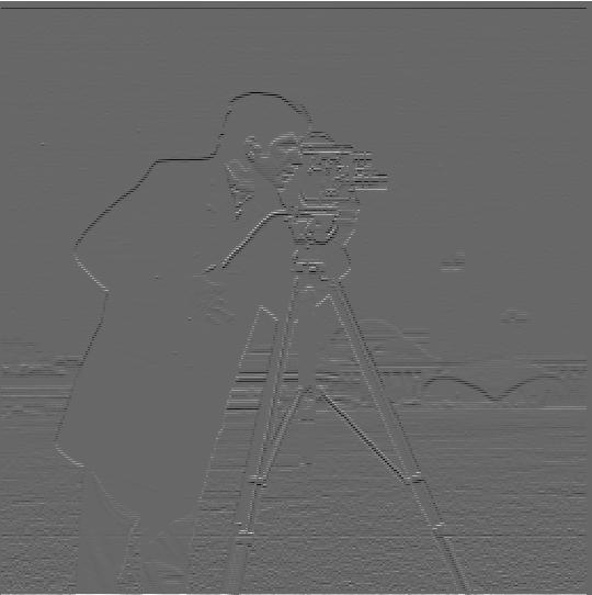
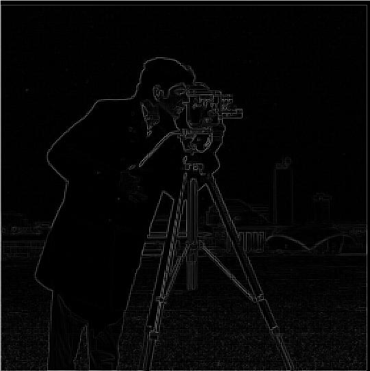
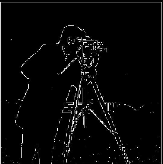
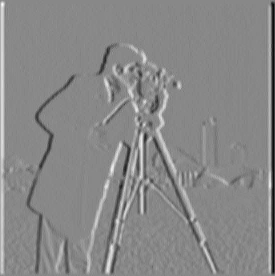
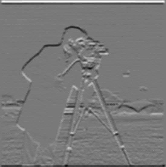
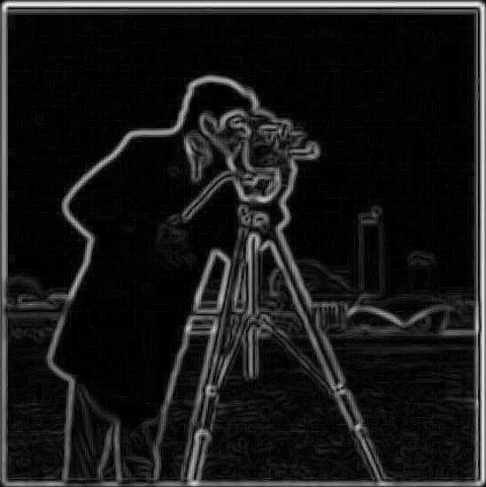
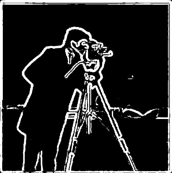
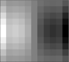
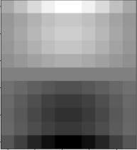
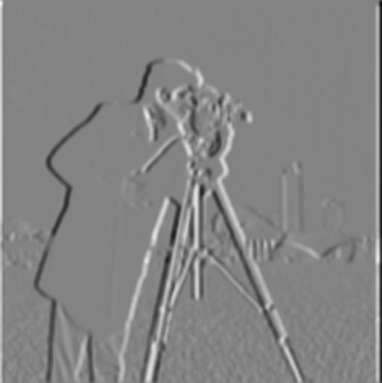
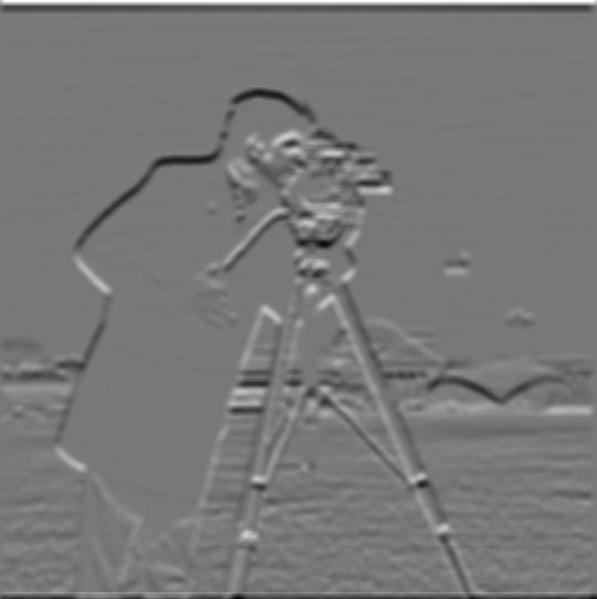
I initially convolved the input image of 'cameraman.png' by convolving it with the mentioned Dx and Dy values from the spec, then used the square root of the sum of the square values of these Dx and Dy values to retreive the gradient magnitude image. Lastly, I took a threshold value of 0.25 to determine the edge image and what values should it consist of (1 if value > 0.25, 0 if less). The images below are Dx, Dy, Gradient Image, and Binary Edge Image (from left to right).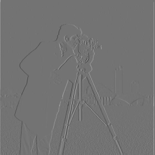

Part 1.2 - Derivative of Gaussian (DoG) Filter

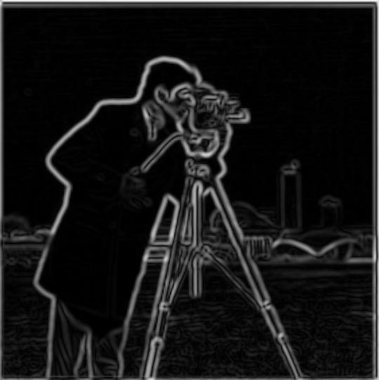
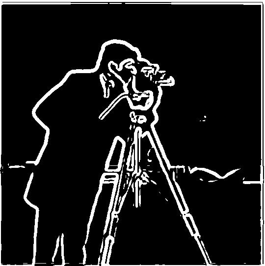
I initially blurred the image using a Gaussian filter and then applied the Dx and Dy operators to retrieve the final edge images. After having compared the results to the ones from 1.1, it's obvious that the edges using DoG are much more visible/evident and intense/amplified compared to the ones from 1.1. The values that I used were: Edge threshold = 0.04, ksize = 10, sigma = 3. The images below are the Gaussian Blurred Image, Dx, Dy, Gradient Image, and Binary Edge Image (from left to right).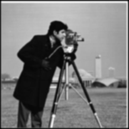



Next, I convolved the gaussian filter with the Dx and Dy values from the spec, which I then used to apply those convolved filters to the image. From just comparing these new results with the results from the first method in part 1.2, we notice that they are essentially the same. The images below are the Gaussian convolved with Dx, Gaussian convolved with Dy, Image convolved with new Dx, Image convolved with new Dy, Gradient Image, and Binary Edge Image (from left to right).

Part 2.1 - Image sharpening

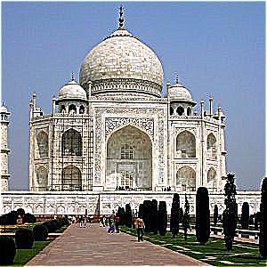
I initially implemented a naive solution where I used a gaussian filter to blur the image, then use this blurred image and subtract it from the original image to retrieve the high frequency image, which I then used to add to the original image to get a final sharpened image. The values that I used were: alpha = 5, ksize = 9, sigma = 1. The images below are taj.jpg and the Blurred Image (from left to right).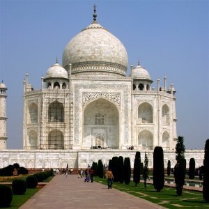



Then, I went ahead and constructed an unsharp filter and applied it to the images.





For an experiment, I took an image, blurred it, and then resharpened it. Since the high frequencies were lost, the resharpened image does not look the same as the original one.

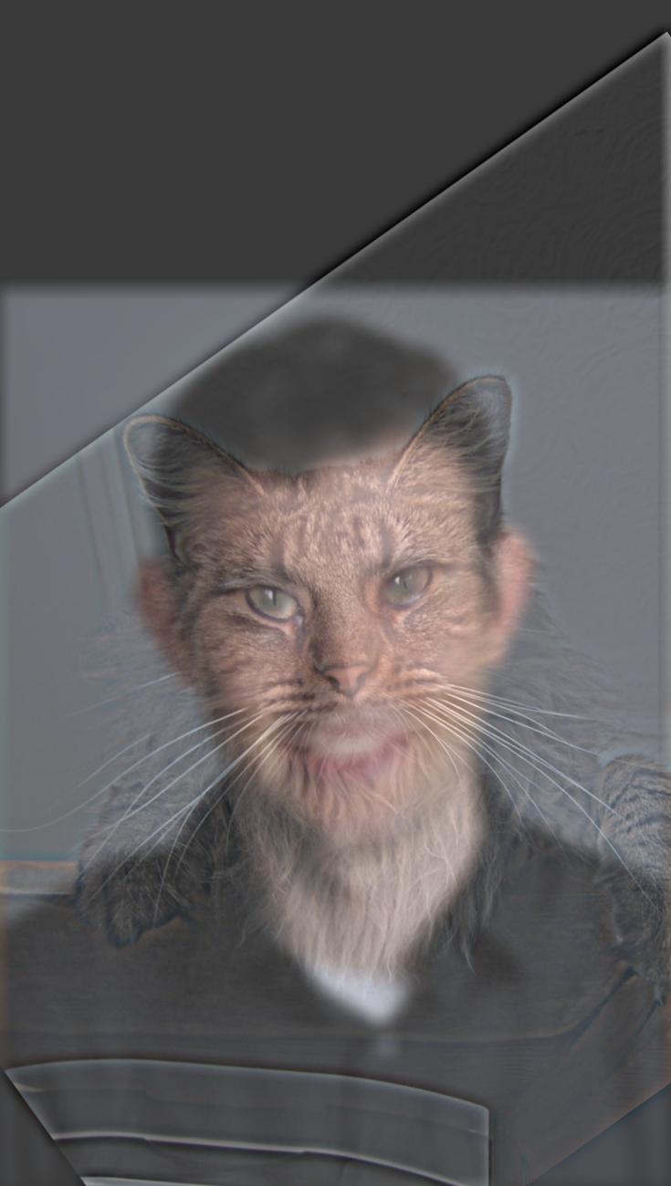
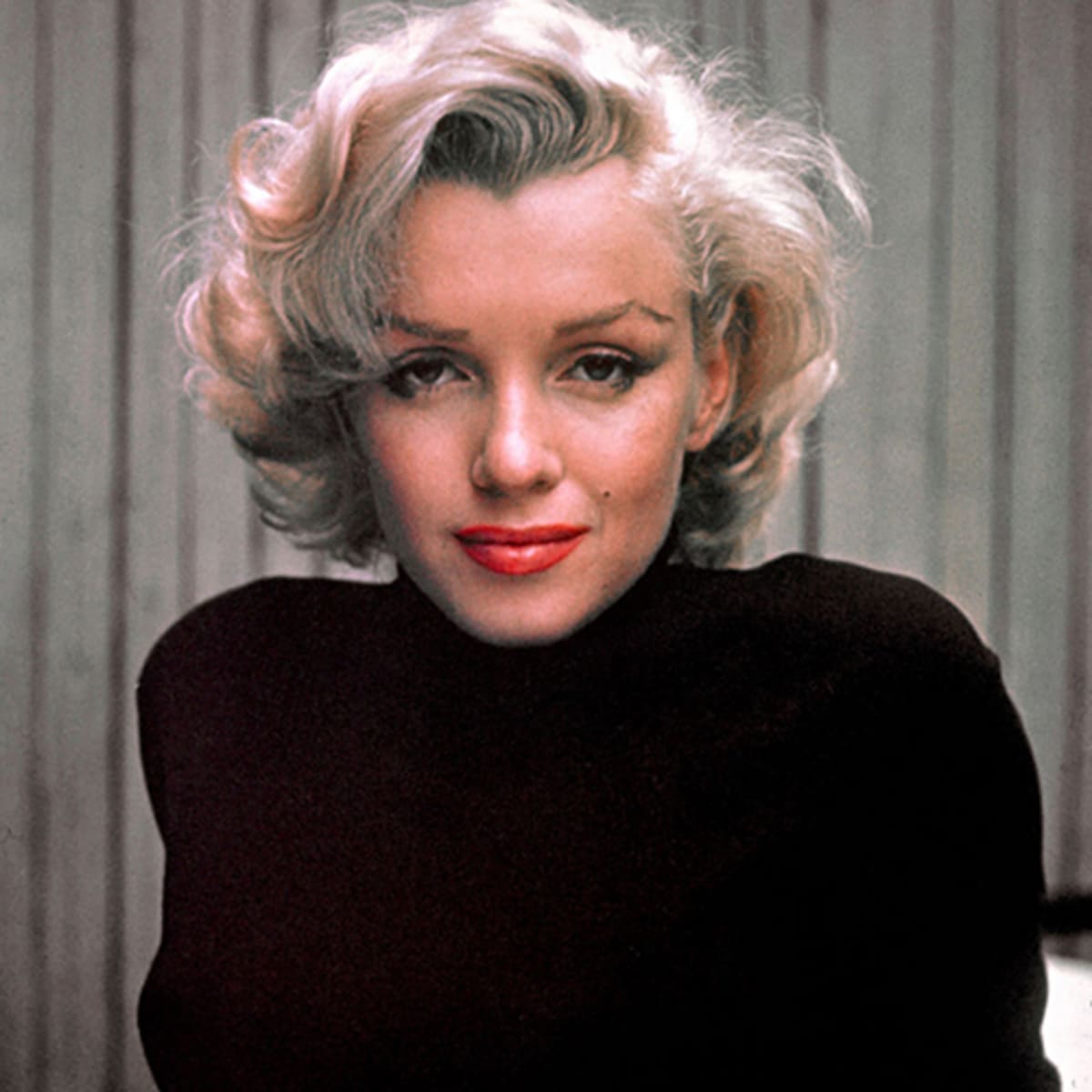
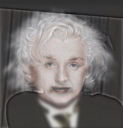
Part 2.2 - Hybrid Images (Along with B&W)

Here are a few examples of the hybrid images that I produced using the method.



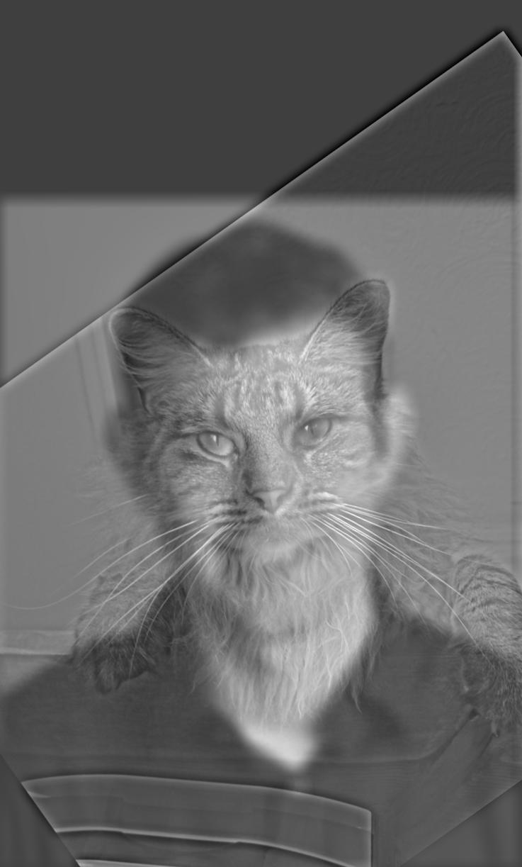
Color obviously enhances the visual perception of the results, and makes the difference between the images much more evident.







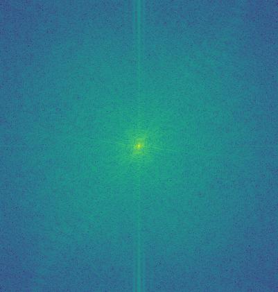
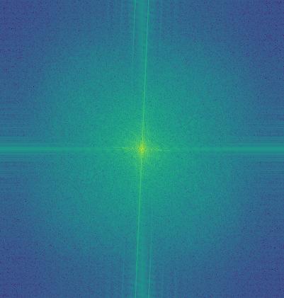
The following images are the log magnitudes of the Fourier transforms of the input images, filtered images, and the hybrid image (from left to right).



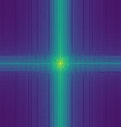
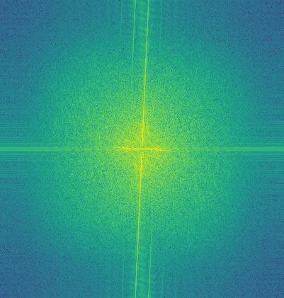
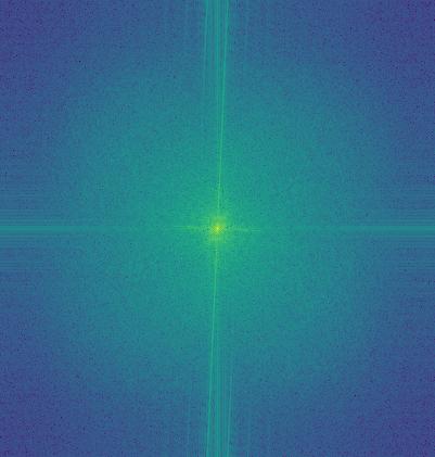
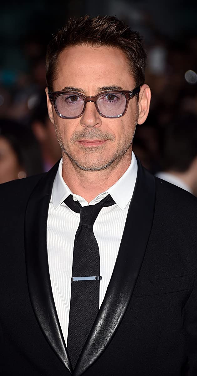
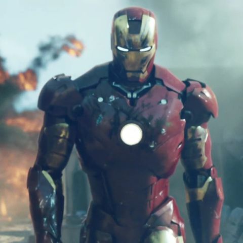
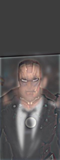
However, not all images work well. A good example is an image of a metallic mask and robert downey jr (metal and face do not mix well!):

We can blend images using laplacian stacks and masking them at each levels, whilst blending at every stack. Using this, we can sum the levels of the stack to get the blended image.

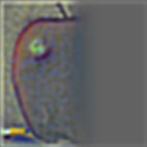
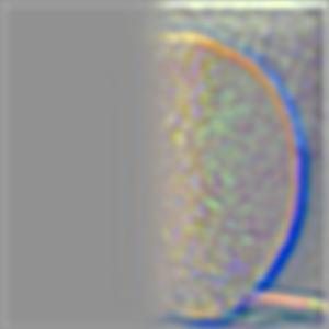
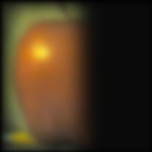
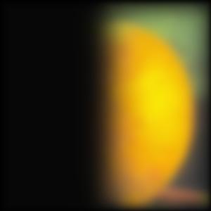
The following images are the laplacian stacks at levels 0,2,4 and the final image for the apple, orange, and oraple.








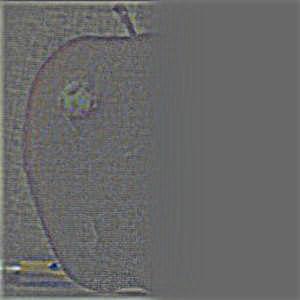
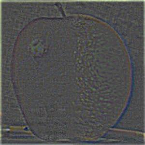
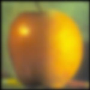
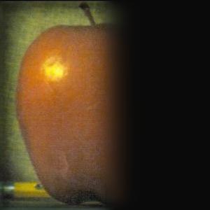
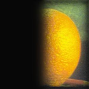
For a black and white image of the apple and orange, we get the following blend:



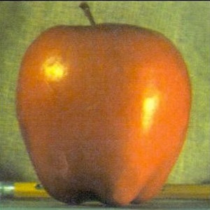
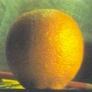
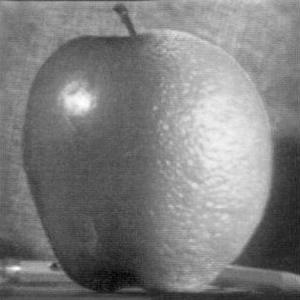
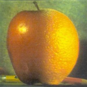
But a colored version reveals much more information (obviously):



Here are a few more examples (with the masks on the far-right side):