CS 294 026 Project 2 Fun with Filters and Frequencies

Author: Tiancheng Sun

Part 1: Fun with Filters

Part 1.1: Finite Difference Operator

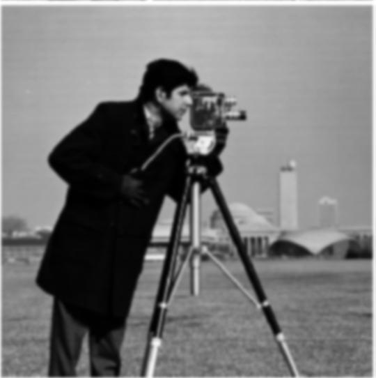
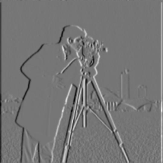
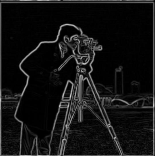
As the first step of the implementation of this naive version of edge detection implementation, I convolved the original cameraman image on with [1, -1] on the x-axis dirextion and y-axis direction sepreately. Since these two images only contains edge on one direction, I combined their information together (via root of square sum quation) and thus obtained the gradient magnitude of the original image. By binarize the gradient magnitude with a threshold of 0.17, the gradient image successfully transformed into a edge image. Below are the results:

The two image in the first row shows the convolution result with dx and dy.

The second row shows the gradient magnitude image its binarized result base on threshold 0.17

Part 1.2: Derivative of Gaussian (DoG) Filter

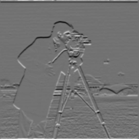
Although I carefully picked the threshold for the binarization process in the previous version of edge detection, the result still seems very noisy and if you look close enough, you will notice that the edge it outlined is basically composed by lots of squares. To obtain a smoother result, I replaced the naive filter with our dear Gaussian filter. The first method is blur the input image first with a 2d gaussian filter first then convolve it again with the two finite difference filter we used in the previous part. Below is the result I obtained:

The first image is the blur result I obtained with kernel size = 12 and sigma = 2, I also tried kernel size = 20 adn sigma = 3, but the it is way too blur and did not give me very decent edge detection result.

The other two image is the convolve result between the blured image and the two finite difference filter

The two image above is the gradient magnitude and binarized gradient magnitude generated base on the Gaussian blured image. The threshold of the binarization process is 0.05

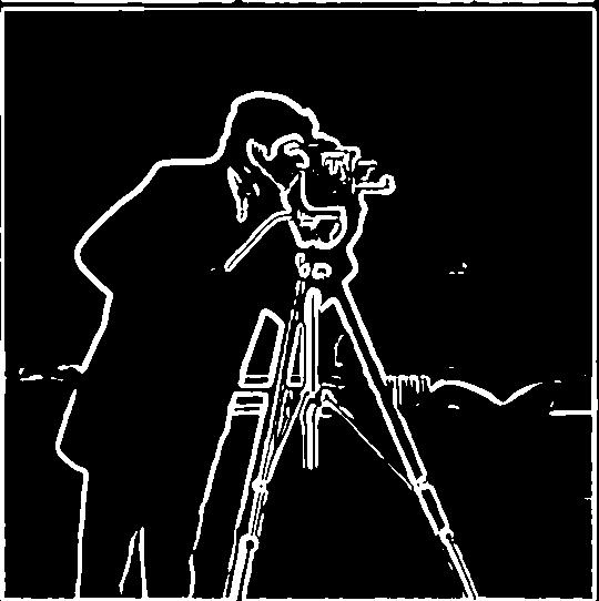
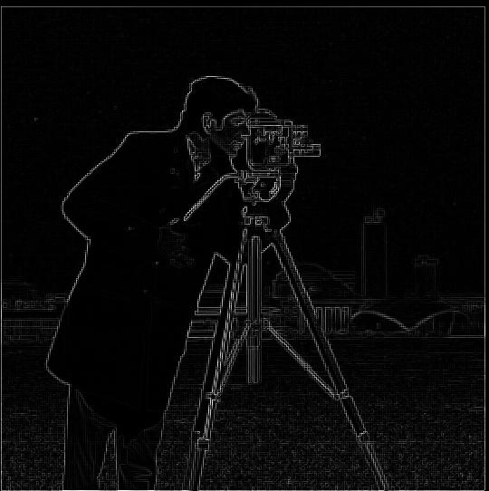
Answer to question 1.2: By compare the manitude image I obtained from part 1.1 and part 1.2, it is obvious to see that with the help of Gaussian blur, the manitude image become much more clean, and the nasty box like partten we observed from the part 1.1 implementation is also disappeared. The binarized edge image also becomes clean and decent even with a much more smaller conversion threshold (0.05 v.s. 0.17)

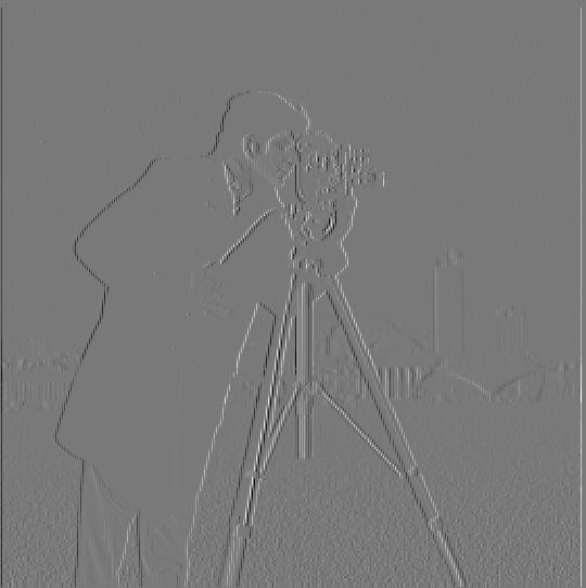
Thanks to the nice math characteristic of the convolution operation, we could combine the previous two convolution together. The result is shown as below, and as we can see the pics is exactly the same with the result we obtained in the previous step:

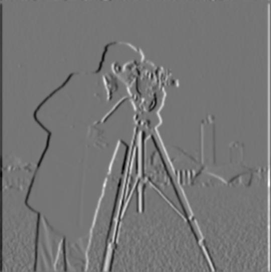
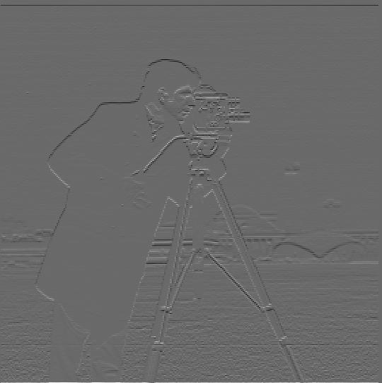
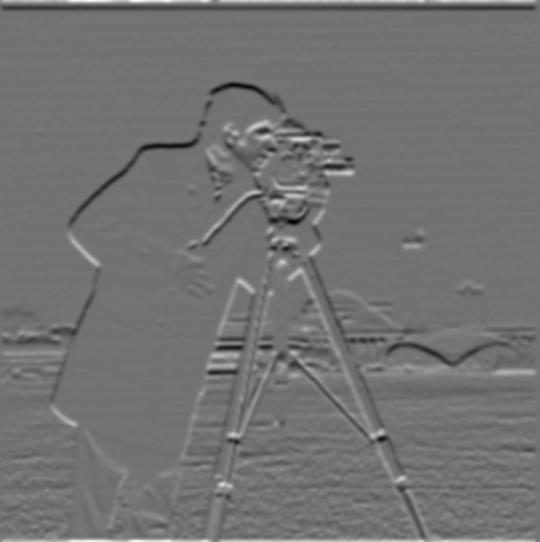Convolution result generated by the original image with DoG filter Gx and Gy

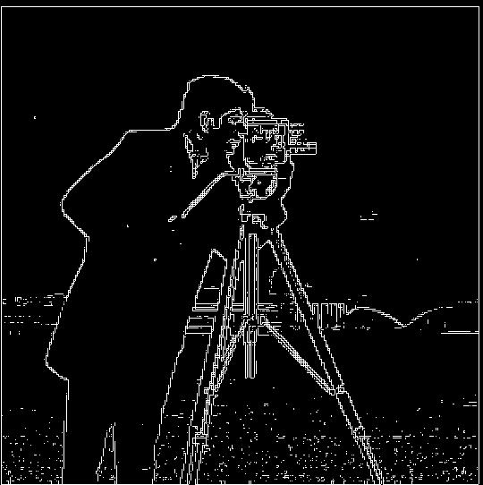
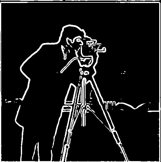Image magnitude generated by the two image above and its binarized version, threshold = 0.05, same as above

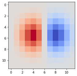
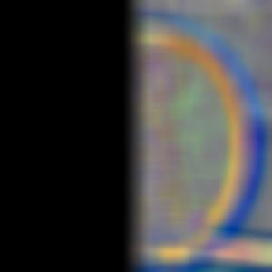
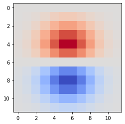The two DoG filter on direction x and y, color mapped to "coolwarm" to show the contrast

Part 2: Fun with Frequencies!

Part 2.1: Image "Sharpening"

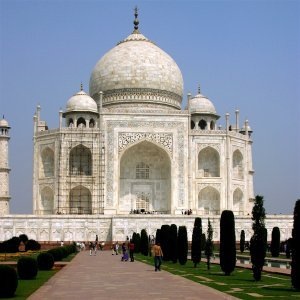
In this part, I took two different approaches to make my blurry image looks more sharp (i.e. add more high frequency detail into the original image). The first one is a more step by step process, I first make the original bulrry image even more blur by convolve with our dear Gaussian filter, then I subtract this low frequency, blured Taj from the original Taj picture and this will allow me to obtain the high frequency part of the original image. By add the high frequency part back to the original image several times allows me to obtain a more sharp image.
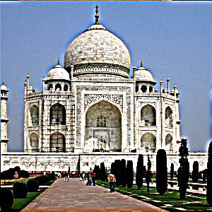
This process is can also be repleced by a signal convolution, the unsharp masking filter. By subtrack the gaussian from the unit impulse (detailed function:(1 + sharp index)e − sharp index * g), we obtained the laplacian of gaussian. After convolve it with the orignal blurry image, we will have exactly the same sharped image as what we obtained from the previous method. Below is a compare between the original taj and the version given by unsharp masking filter:

original Taj image and the sharped version

Here is one more example I piced from my cell phone albumn:

As request, here is an example of sharp img, blur, and resharp:

By compare the orignal high resolution image with the fake sharp image I produced, it is easy to identify that the resharped image lost lots of details and become quite noisy. In the original img, there are quite a lot of nice "pure" color part, but they become dirty in the resharped image. ### Part 2.2: Hybrid Images Since human's vision tends to focus on high frequency information when its avaliable. We could belnd two image together into different frequency range to make people stand at different distance to the image see different content. To do this, I use high-pass fiter processed the cat and use low-pass filter processed the man:

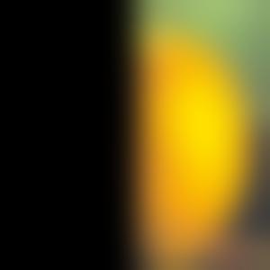
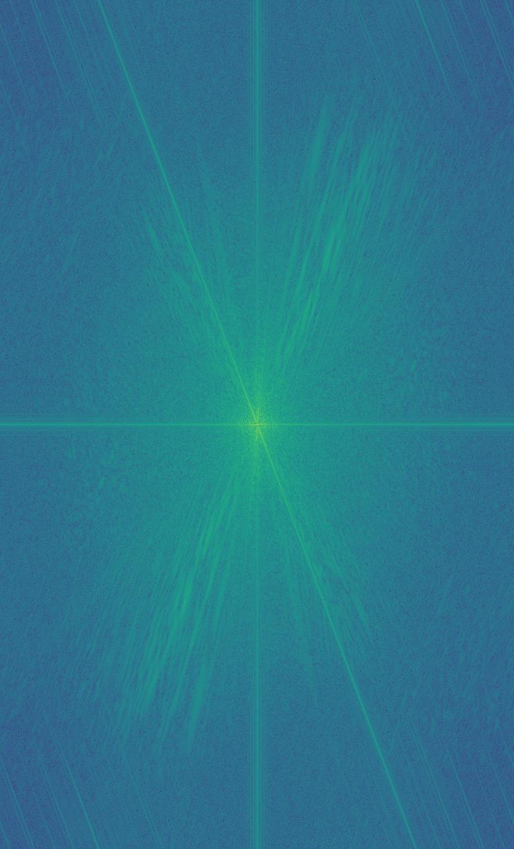
>>>low pass>>>

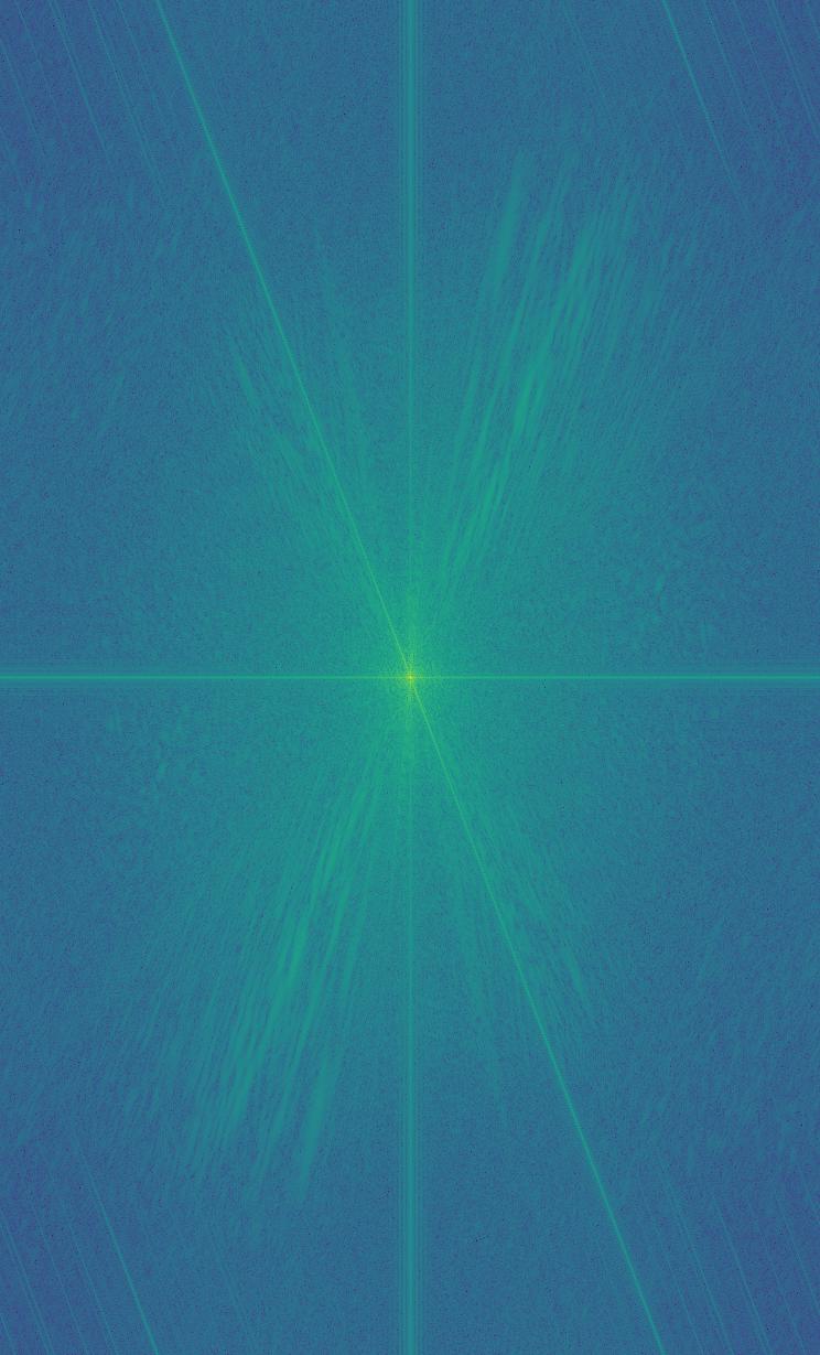
>>>high pass>>>

And here is the result:

The low pass filter's sigma is 40 while the high pass's is 500, so that I could save as much info from the cat image as possible.

Below is the frequency analysis result:

From left to right, there are the Fourier transform of the two input images, the filtered images(low -> high), and the hybrid image

Here are more examples of blend images made by me:

And here is an failed example:

After analysis, I think the reason account for this failure is the fact that this two image is not "different" enough, so even they are blended together, people cannot tell

Multiresolution Blending (a.k.a. the oraple!)

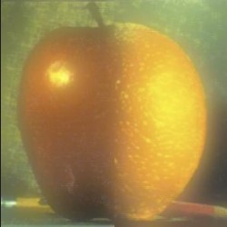
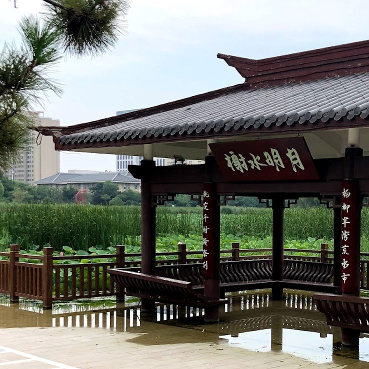
For this part, the kernel size I choose is 30 and the sigma is 15; I taked a slightly sifferent order compare with the original algorithm published on the paper to blend the gaussian blured mask and the laplacian stack, so in below the color is slightly different with the original paper, but the blend result is still good:

The first two row demostrated the Laplacian stack at different frequency (from left to right, high, mid, and low), the last row is the blend result