CS 194-26: Fun with Filters and Frequencies!

Amol Pant

Part 1

Part 1.1

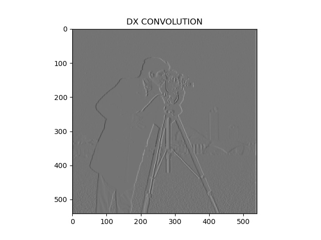
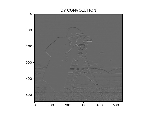
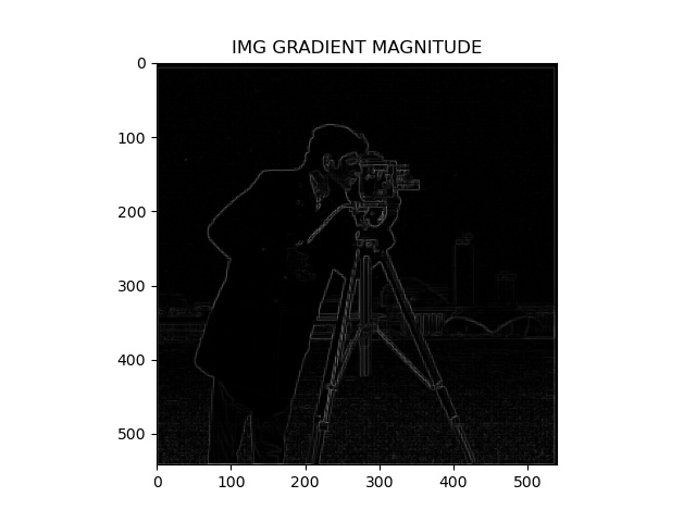
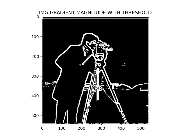
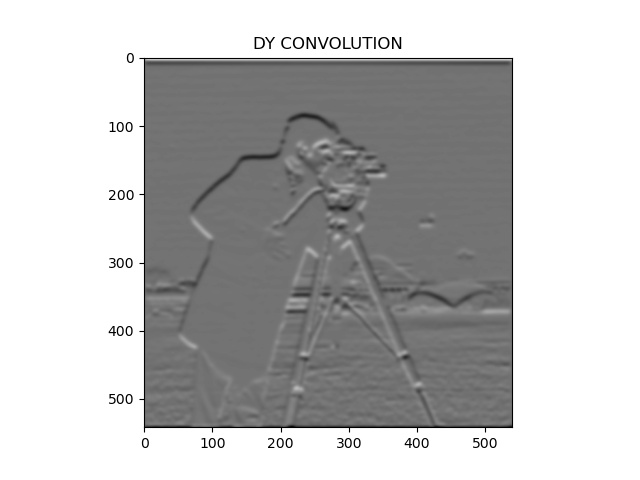
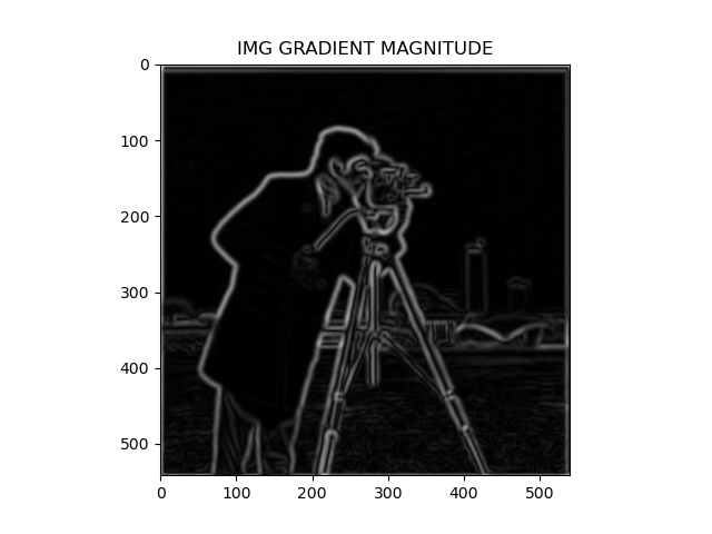
For my baseline function, I first did dx and dy kernel convolutions on the given image. We then combine our results to find the gradient magnitude image.
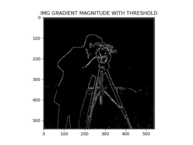
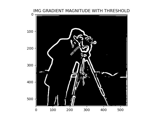
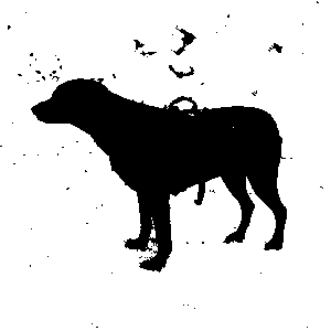
If we pass this gradient image through a threshold filter, we get a rough idea of edges on the image and it essentially functions as an edge detection filter on the original image.
Here are the results of that basic image operation pipeline:

Part 1.1 Images

Original	Basic DX Filter	Basic DY Filter	Gradient Magnitude Image	Gradient Image With Threshold

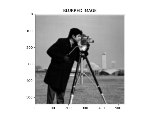
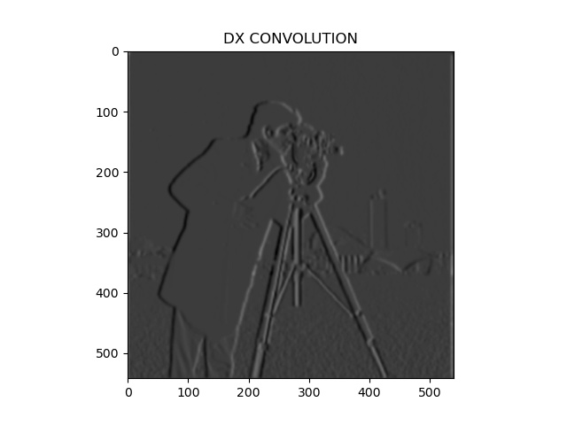
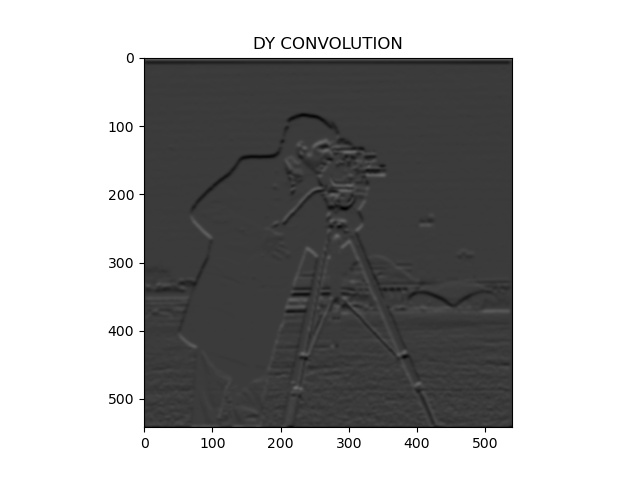
However, the edges look rugged and not smooth like in real life. To make this edge image look like a drawing, we can do the same process as above after blurring the original image by convoluting it with a 2d gaussian kernel. Then I blurred the image and did the same process. Here are the results:

Part 1.2 Images

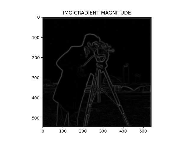
Blurred	DX Filter	DY Filter	Gradient Magnitude Image	Gradient Image With Threshold

Notice how the edges of the image at the end are much more smoother and are a better way to depict the edges of the original image.
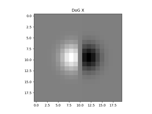
Another way to get the same result is to convolute the kernel itself rather than the image, since linearity allows changing order of operations making operations more elegant sometimes.
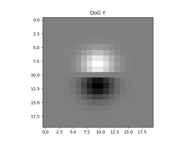
Here are the Derivative of Gaussian (DoG) filters which we will use as our new kernels:

DoG X	DoG Y

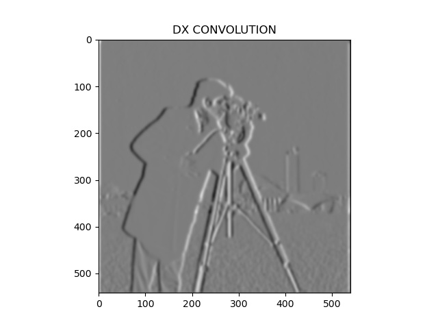
And here we have the results of using these kernels:

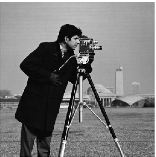
Cameraman	DoG X Filter	DoG Y Filter	Gradient Magnitude Image	Gradient Image With Threshold

Here we can notice that the output image is very similar to that if we had blurred the image first.

Part 2: Fun with Frequencies!

Part 2.1

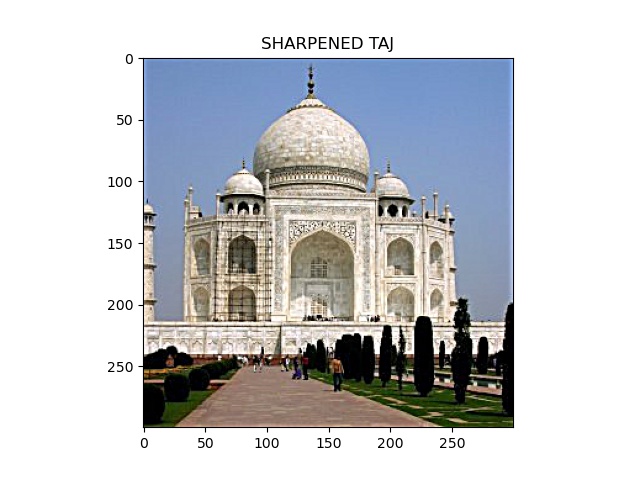
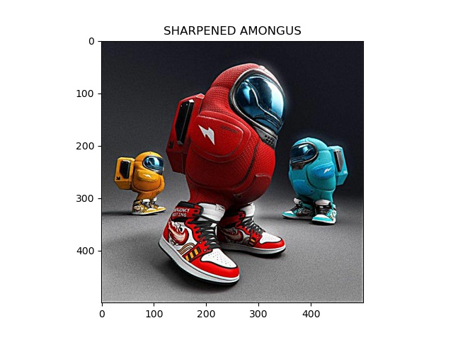
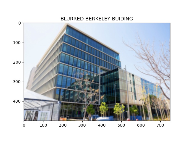
Our objective is to sharpen up an image by essentially adding some high frequencies to the image.
The naive way would be to first find the gaussian, subtract the gaussian from the original, and add the subtracted to the original.
However, we can change the order of operations and instead have a single convolution with the "unsharp filter" work for us.
Here are the results of using the unsharp filter.

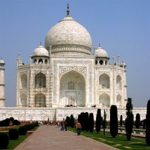
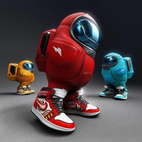
Original	Sharpened

Original	Blurred	Blurred then sharpened

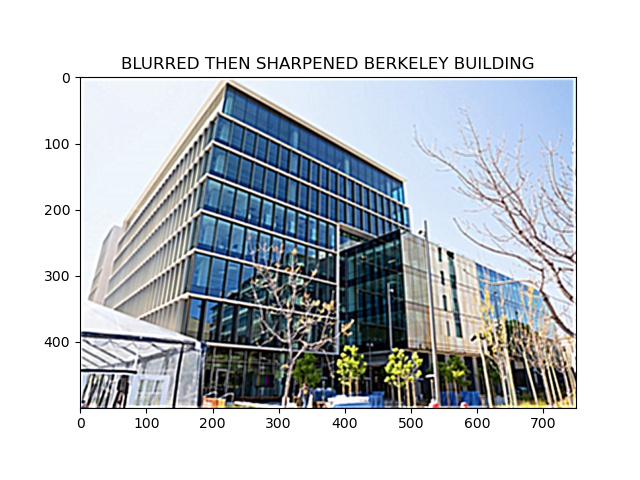For the last one, we tried blurring the image and then resharpening it. Although it looks okay, there was definitely some information lost in the process.

Part 2.2

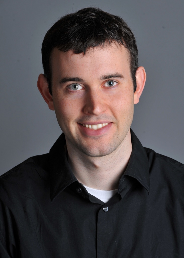
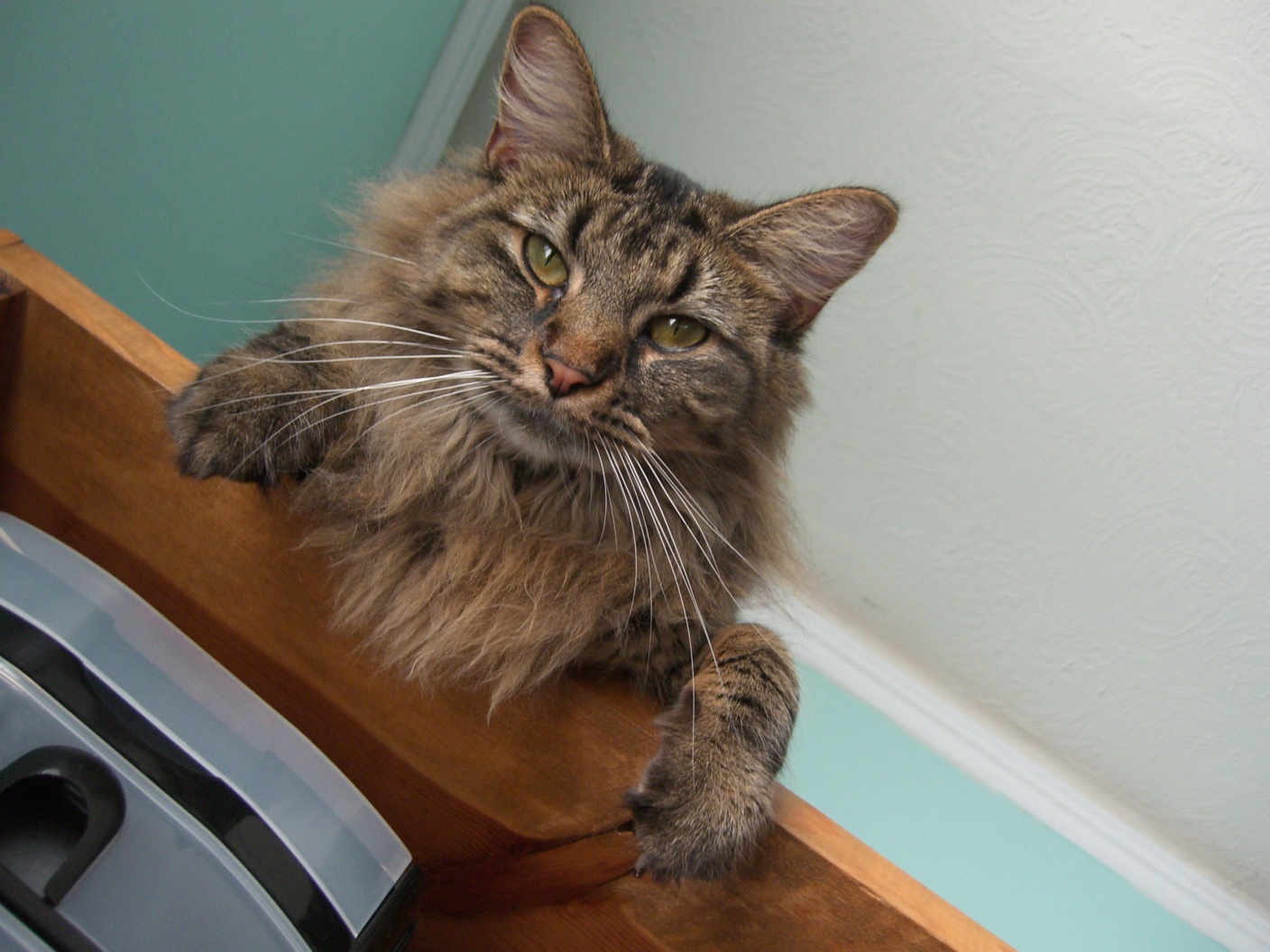
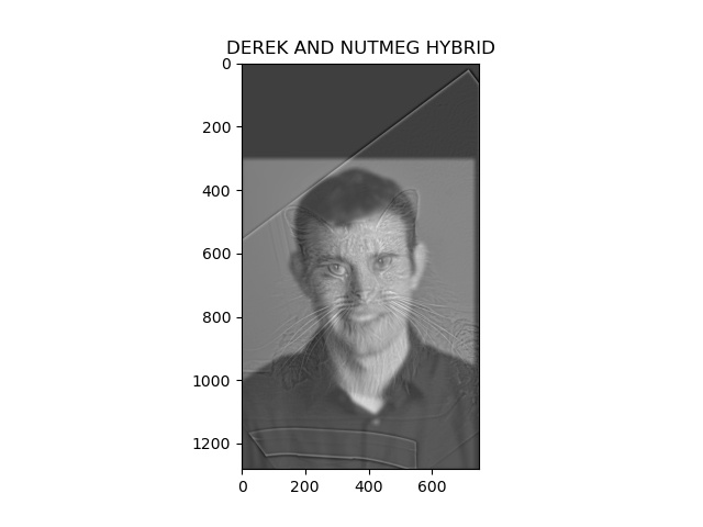
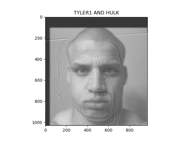
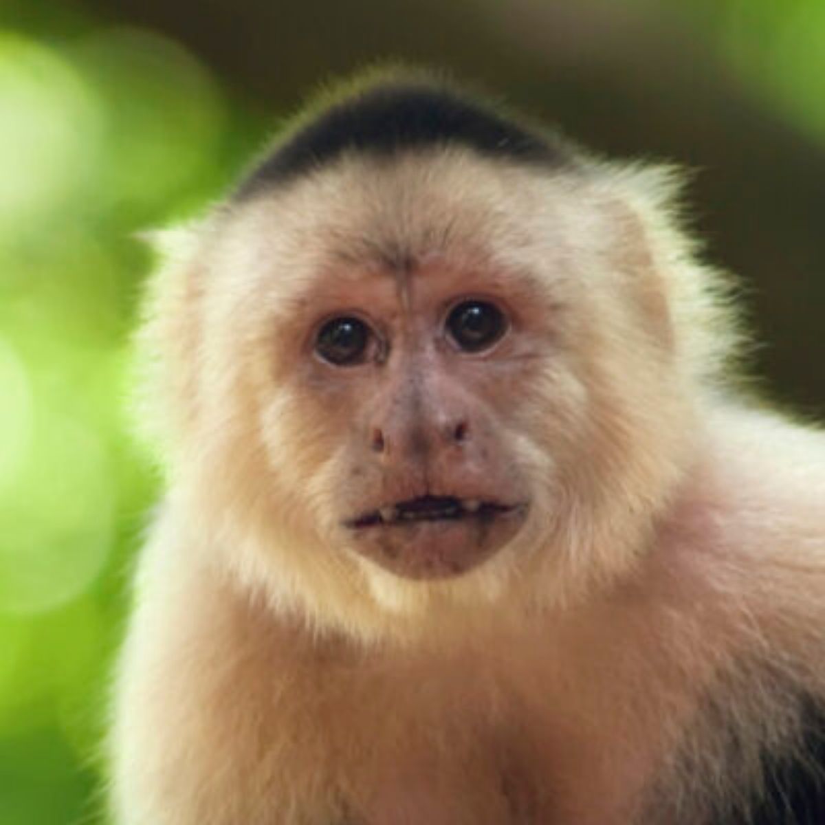
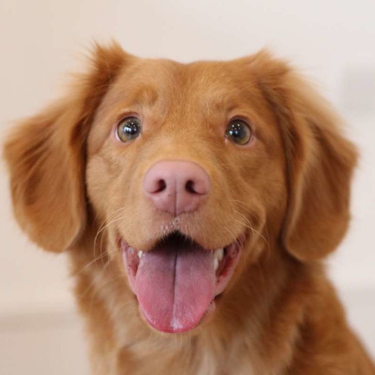
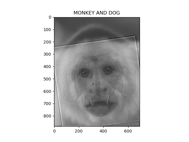
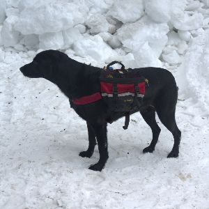
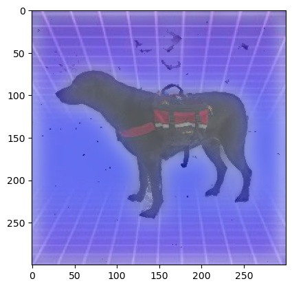
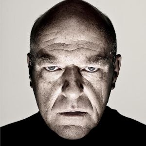
Now we will try to make some hybrid images by aligning 2 images, and merging the low frequencies of one with high frequencies of the other.
Here are the results:

Image 1	Image 2	Hybrid

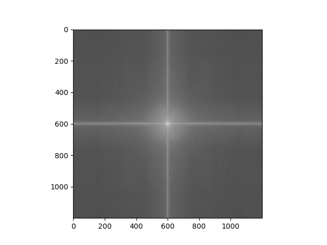
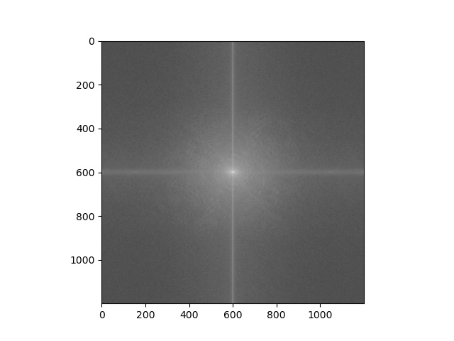
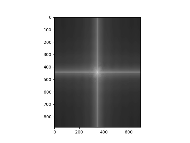
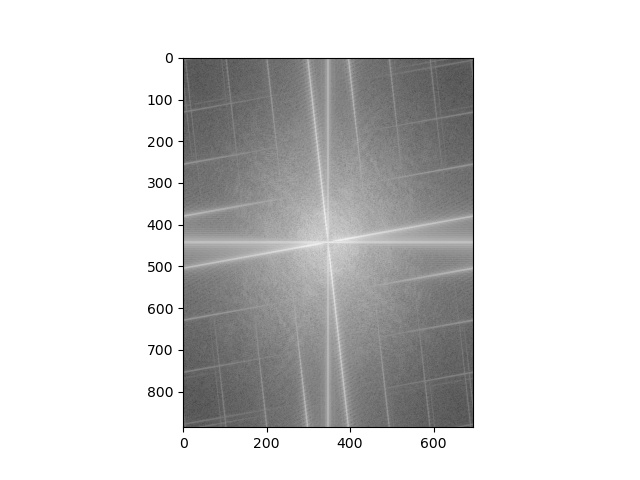
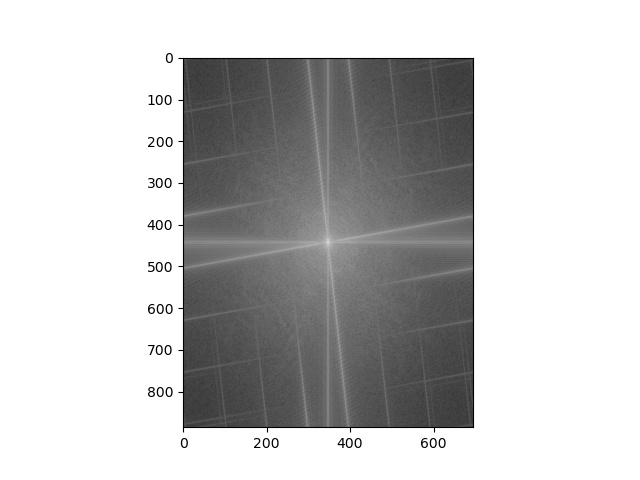
For monkey and dog, we can walk through the merging process in the frequency domain by performing fft at each step:

Image 1 fft	Image 2 fft	Image 1 low fft	Image 2 high fft	Hybrid fft

Part 2.3

Now we will try to take 2 images and blend them together with a seam. This seam will be represented by a mask that we do on the first image and inverse mask we do on the second.
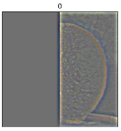
The idea is to create gaussian stacks by repeatedly gaussian blurring and stacking the results. We also make laplacian stacks by subtracting each level by the next of the gaussian stack.
With these low and high frequencies of the mask and the images, we can add each level and sum them up to get a blend of images.

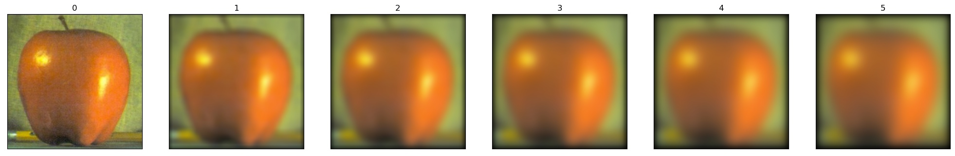
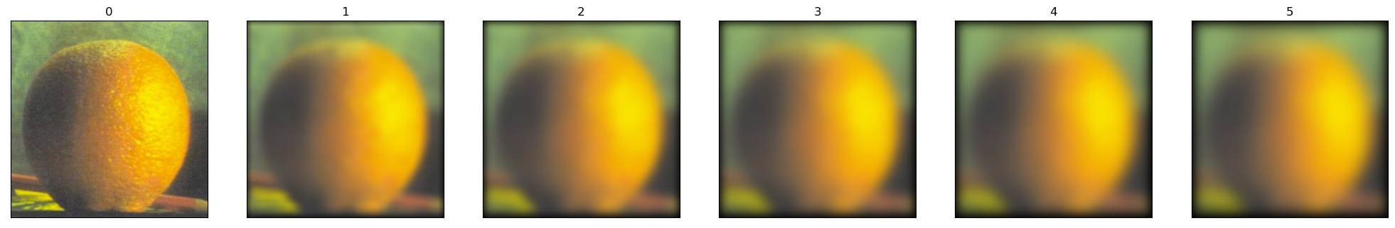
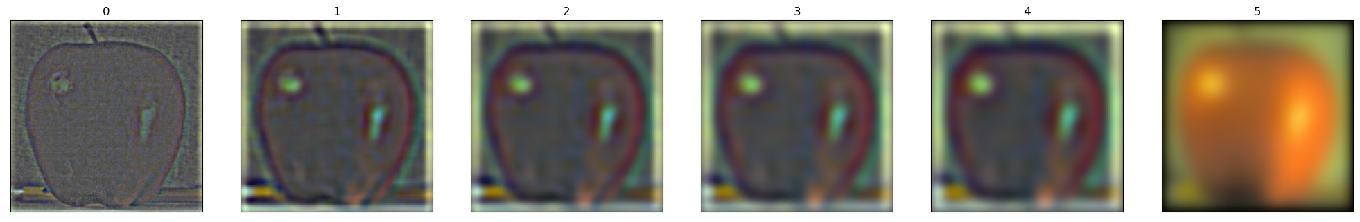
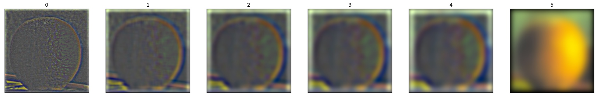
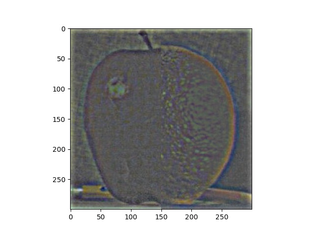
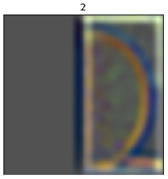
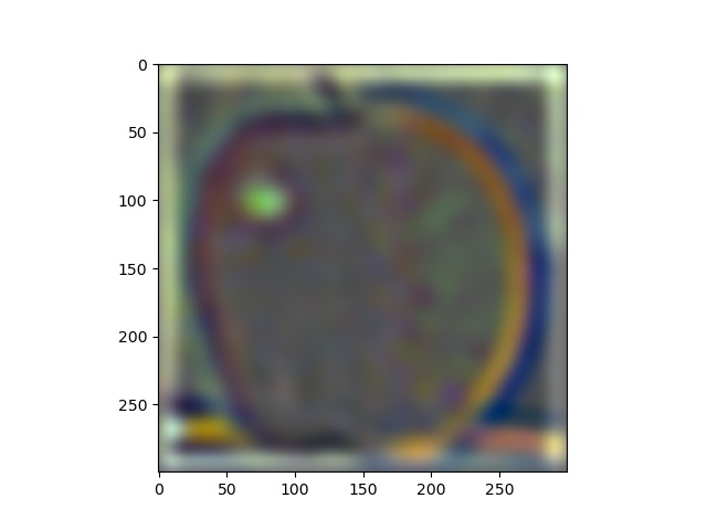
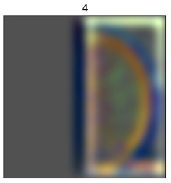
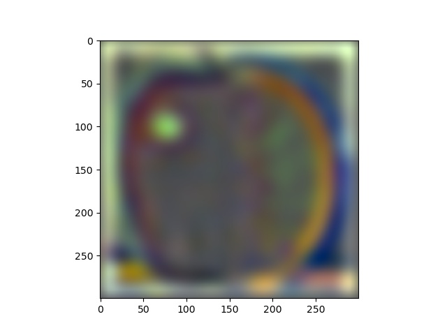
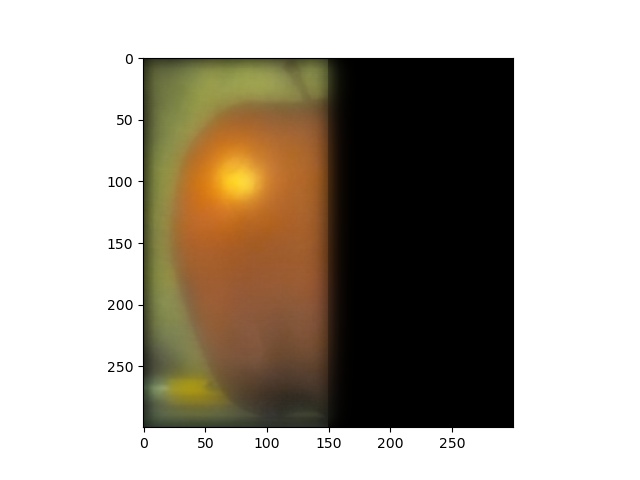
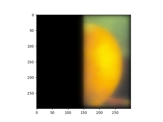
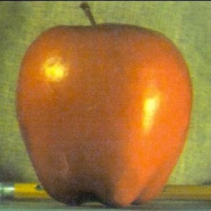
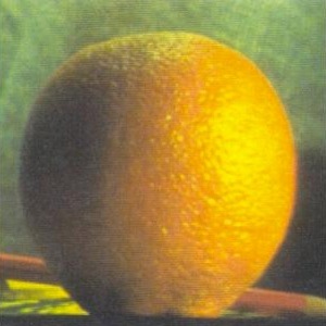
Lets begin by first taking an apple and an orange and showing their gaussian and laplacian stacks.

Image	Gaussian Stack

Image	Laplacian Stack

Now we can try to recreate the figure 3.42 from the textbook by taking small snapshots of the intermediate processes from levels 0,2,4 of the stacks.
I personally took screenshots from the laplacian stacks I made at levels 0, 2, and 4 for the first 3 rows

Apple	Orange	Blend

Part 2.3

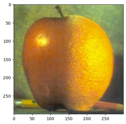
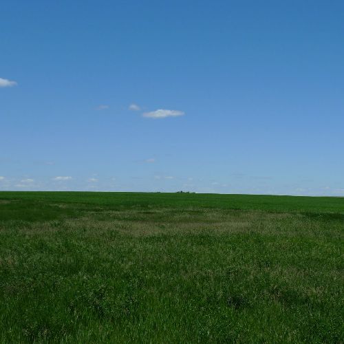
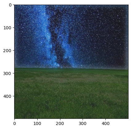
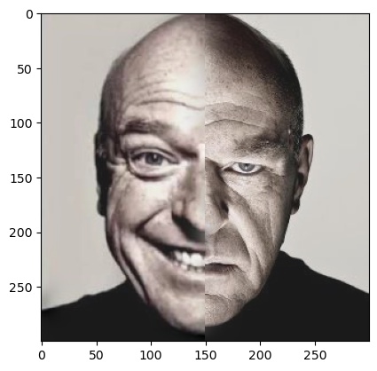
Here are some exmaples of blending images. For some I used a basic mask and for some I used a custom mask so that the edges blend better.
The main improvement of laplacian blending over direct masking is the brightness values and how the brightness doesnt change too much when going from 1 image to the other.
For the final image, the line can be more distinctly seen since a basic mask is used on more complicated subjects.

Image 1	Image 2	Mask	Blend