In this project, we will be 1) applying 2D convolutions and filters to images to better understand these operations' properties and 2) playing with frequencies to sharpen images, build hybrid images, and blend images together.
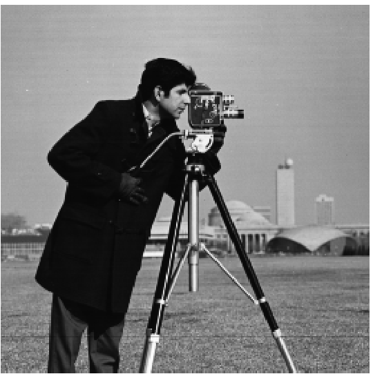
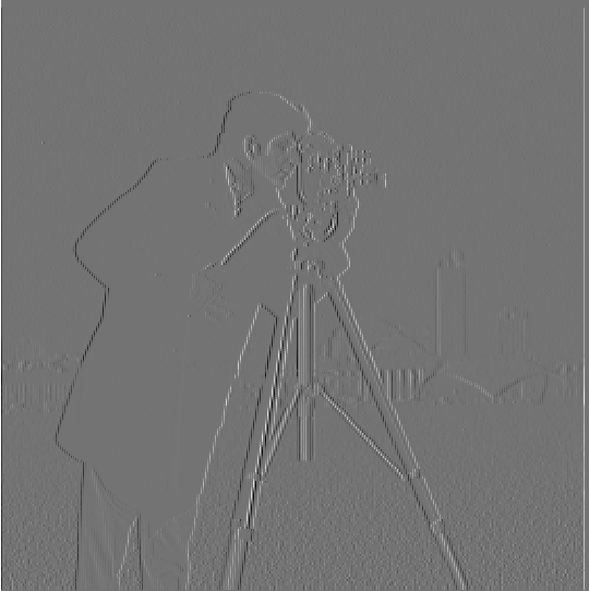
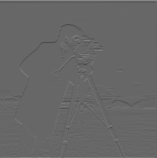
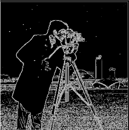
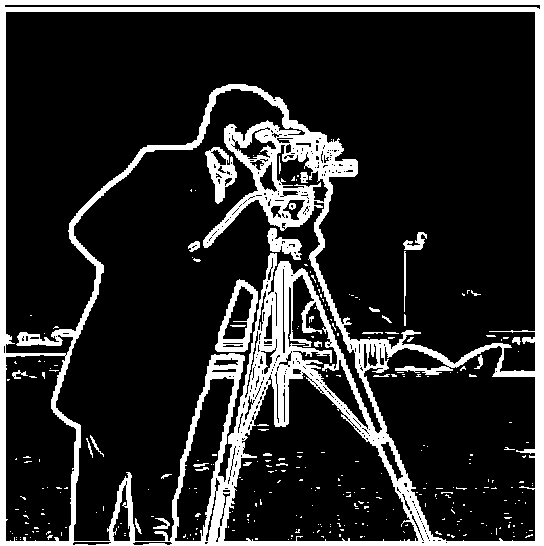
In order to compute the gradient magnitude, as we do in this subpart, we first take the partial derivatives with respect to x and y of the cameraman image we were provided. We compute these partials by convolving the image with our filter (in this case, our finite difference operators). Then, we take a dot product of each partial of the image with itself, sum these squares of partials, and take a square root to get the gradient magnitude matrix / image.
Here is our step by step process of computing the gradient magnitude image (as well as binarizing it).
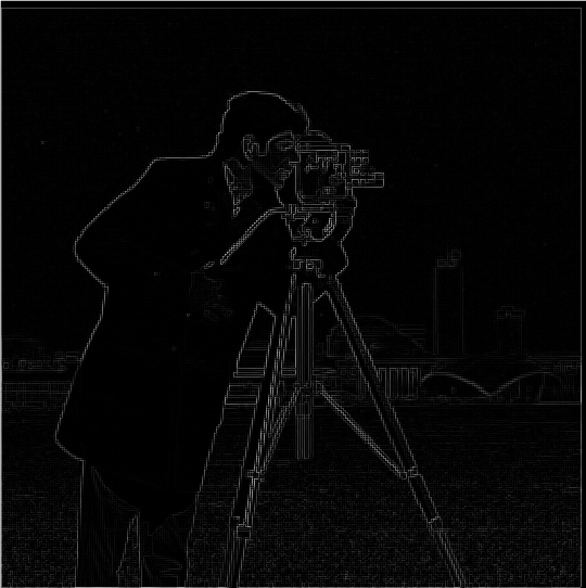
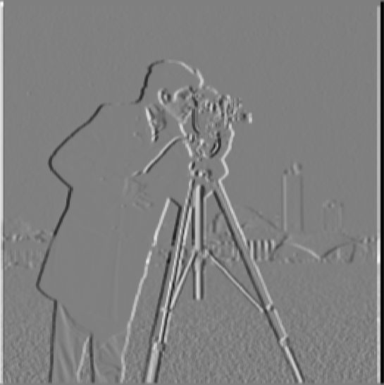
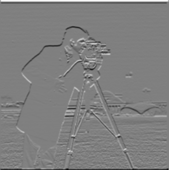
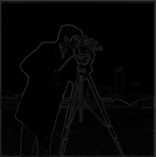
We notice that our final result in Part 1.1, despite containing many of our desired edge lines, has a fairly large level of noise. In this part, we are going to construct convolve our Gaussians with our finite difference operators to construct DoG (Derivative of Gaussian) filters. Compared to our prior images, we will see that the final edge image we get from this approach has less noise and that the partials we compute along the way seem to have stronger countours. Furthermore, in the project notebook we have verified that the result we get using the DoG filters would be the same as the result from first convolving the image with the Gaussian and then with the finite difference operators (rather than the Gaussian first with the operators and then the image with that, as in the DoG case).


In this subpart, we'll take a blurry (low frequency) image and "sharpen" it by finding the image's higher frequencies and then adding these higher frequencies in to the degree necessary for the image to look "normal". We can get these higher frequencies of the image by first convolving the starting blurry image with a Gaussian to get an even blurrier image, which would then contain the "lowest" frequencies, and subtracting these "lowest frequencies" from our original blurry image to get the high frequencies.
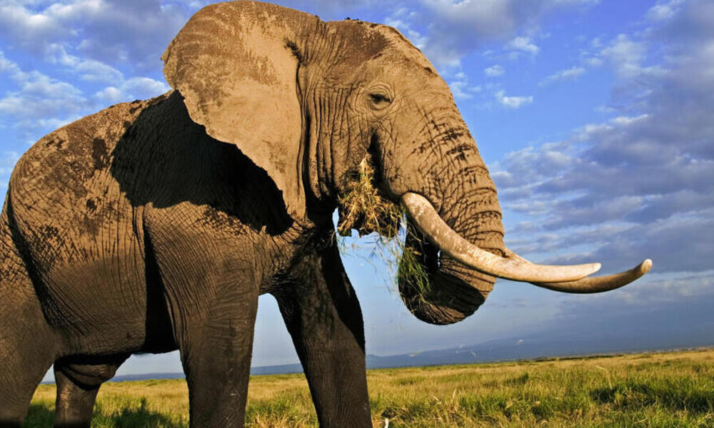
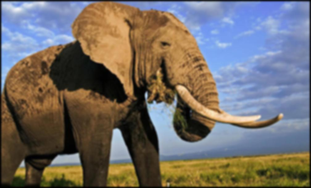
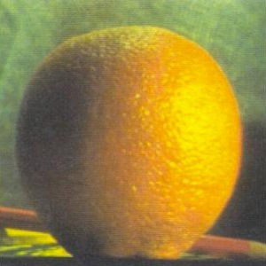
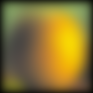
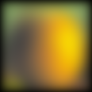
This elephant image doesn't really need sharpening, so we'll blur it a bit first and then see if we can recover the details using our sharpening algorithm! Source of elephant image: https://www.worldwildlife.org/species/elephant

You can see that the sharpened image here looks a bit less smooth / a bit higher contrast as compared to the original, which perhaps follows from the "loss of information" from blurring in the first place.
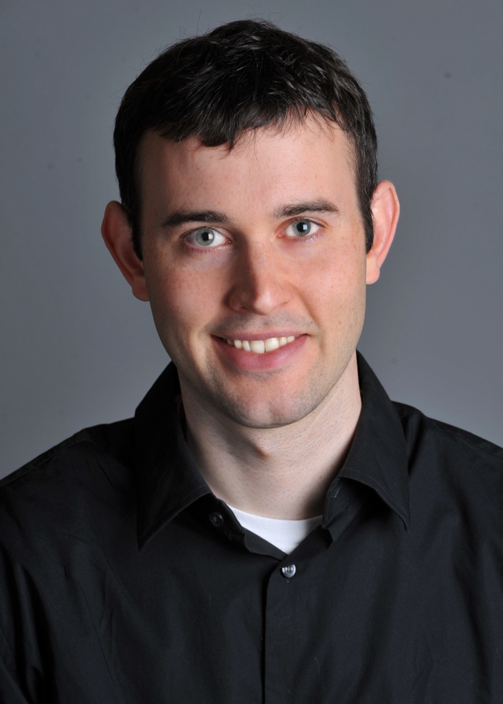
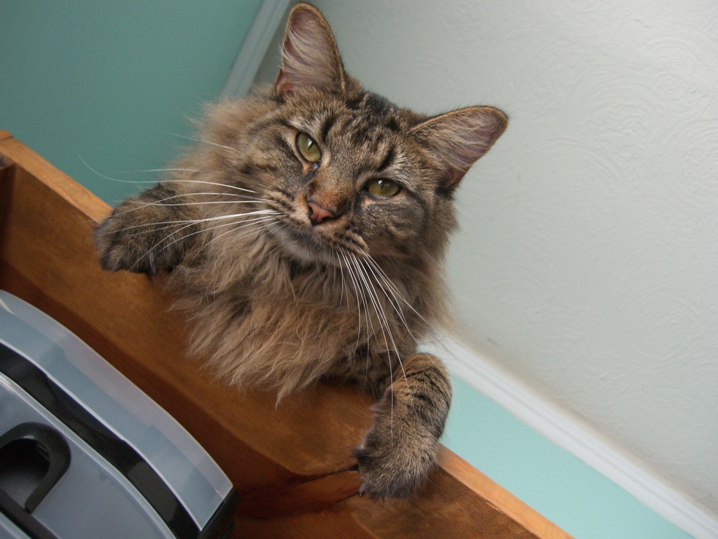
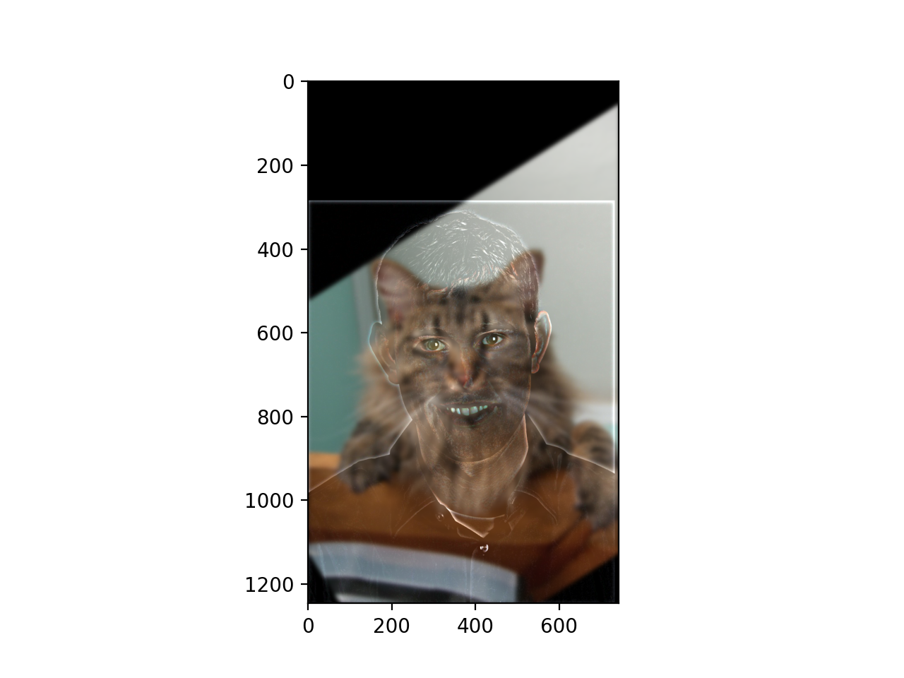
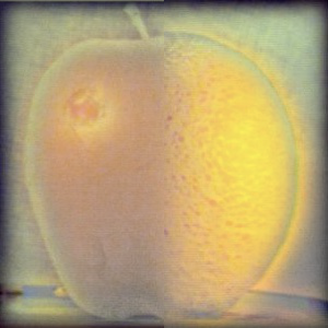
In this part, we will create hybrid images (images that look different from nearby versus faraway) through manipulating the frequencies of each of our images that we're combining. Our first example features a hybrid image of Derek and his former cat, Nutmeg. We construct our hybrid image by retaining the low frequencies of Nutmeg and the high frequencies of Derek and combining them. The result is an image which looks like Derek from nearby but Nutmeg from far away.
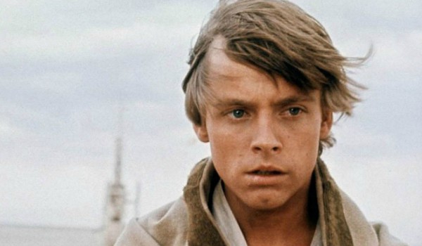
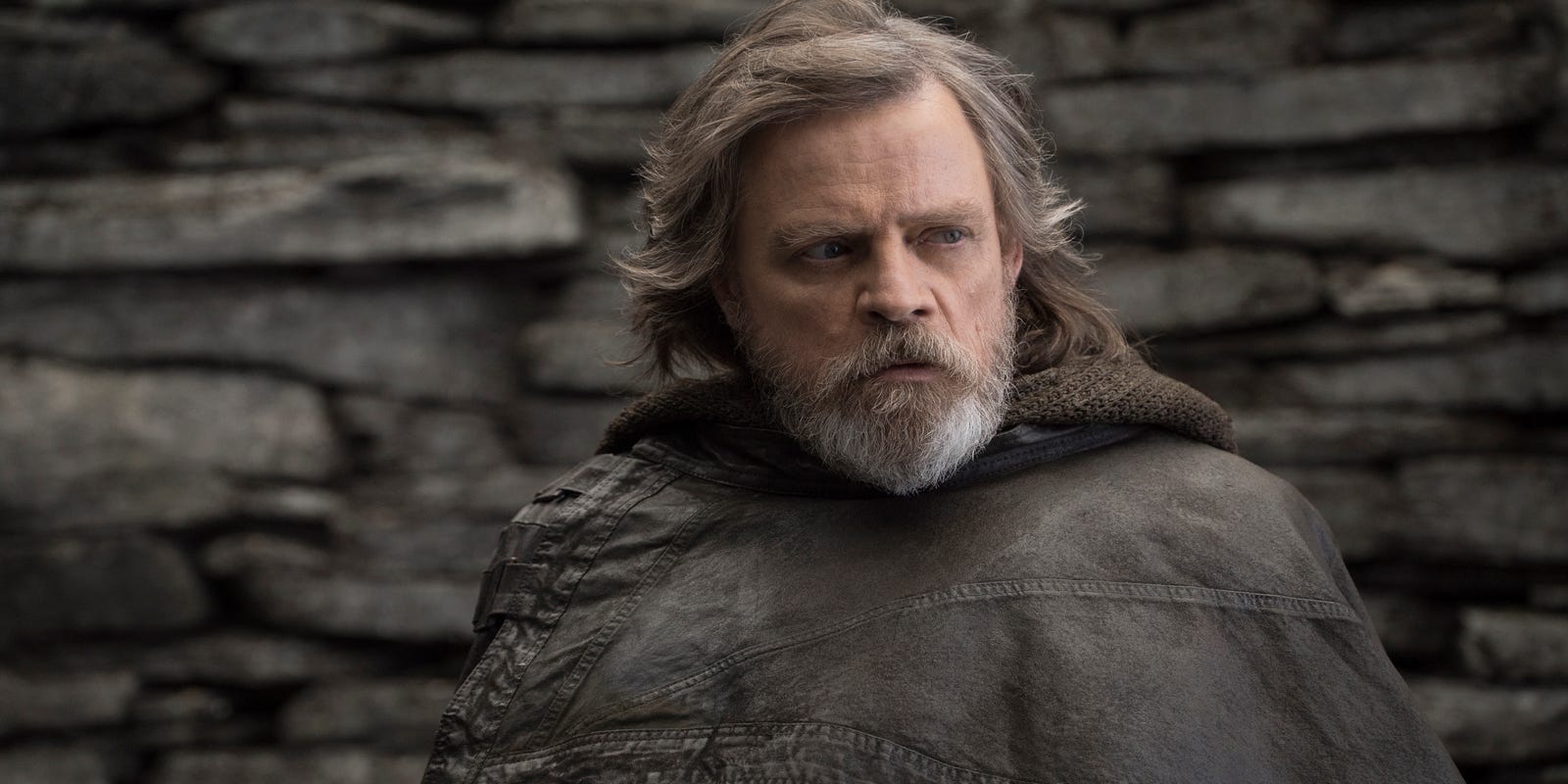
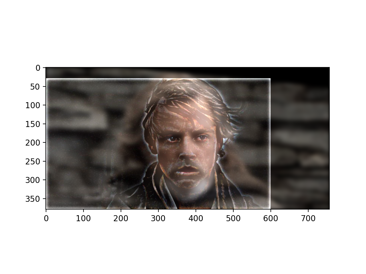
We can try our new hybrid_image function on other combinations of photos, as well! One that I really enjoyed was combining an old Luke Skywalker with young Luke Skywalker (he still looks the same to me). Image credits for Young Luke (1) https://www.cinemablend.com/new/One-MCU-Actor-Looks-Exactly-Like-Young-Luke-Skywalker-Check-Insanity-Out-130247.html and Old Luke (2) https://www.usatoday.com/story/life/movies/2017/12/10/wiser-mark-hamill-still-having-galactic-fun-old-luke-star-wars-last-jedi/932573001/
From nearby the hybrid image, we now see Young Luke, and from far away, we see Old Luke.
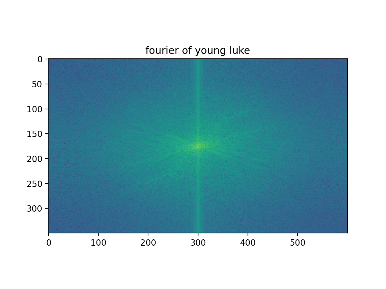
This one was a favorite of mine, so we can look at the results in Fourier space, too.
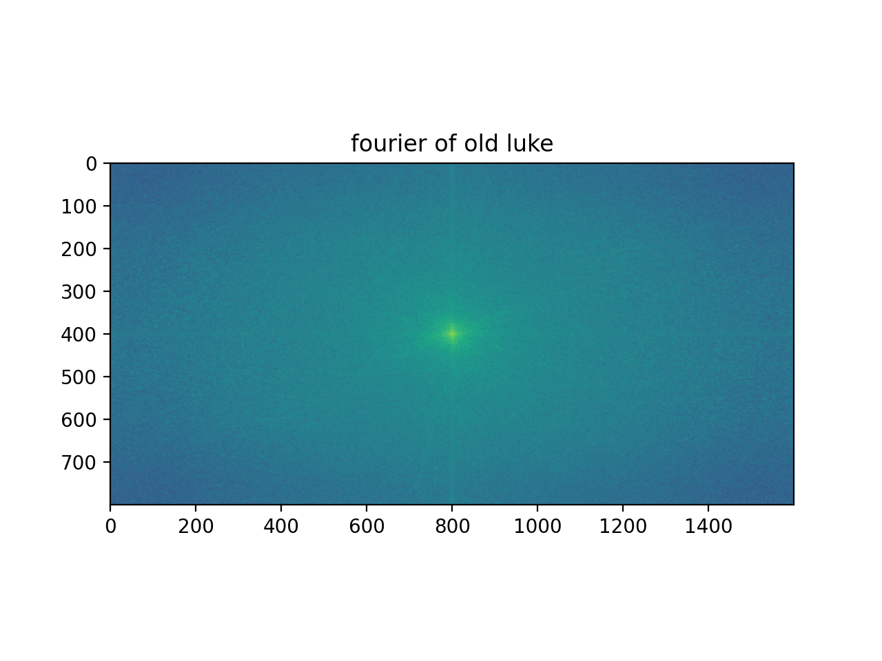
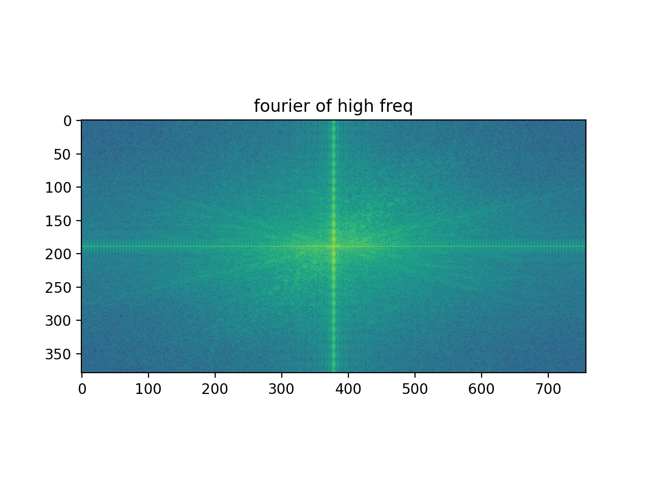
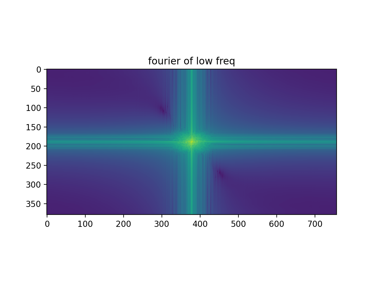
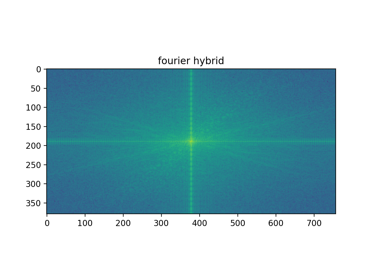
One thing worth noting here is that our Old Luke image (which we took low frequencies from) and our Young Luke image (which we took high frequencies from) already had frequency distributions similar to what we had sampled them for (i.e. the Old Luke image was not a lot of high freq and the Young Luke image had a good number of high freq). This made the job of combining them simpler and the result was a fairly strong hybrid image.
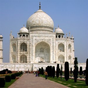
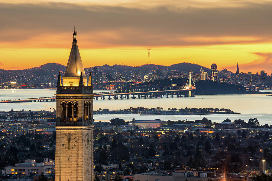
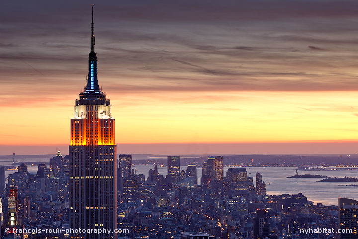
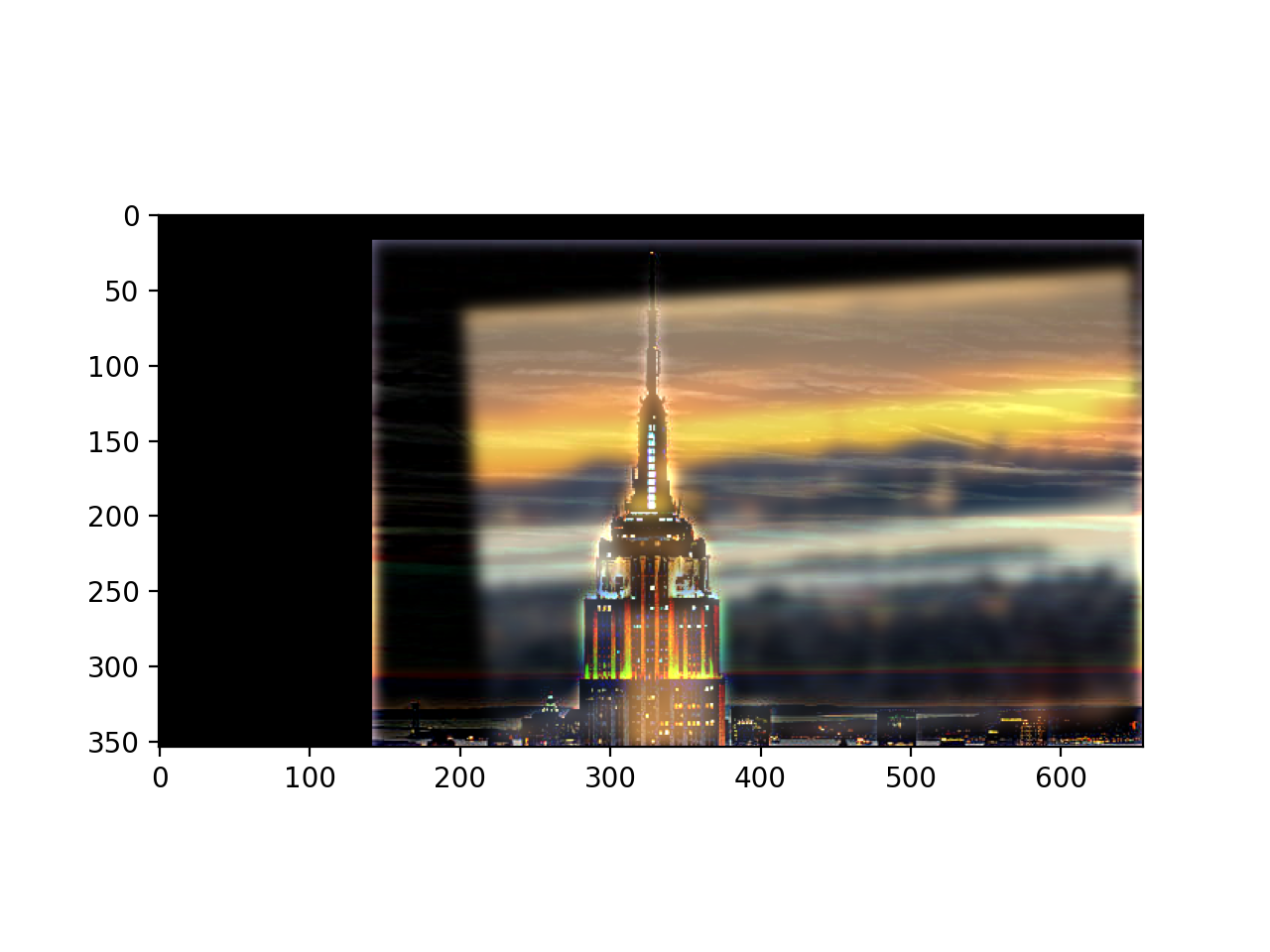
The following example is not as great of an example of a hybrid image, primarily because the starting images we use of the Campanile and the Empire State Building are both high in frequency and contrast, so when the Campanile gets blurred (i.e. through our low pass filter), a lot of the information is lost. Credits for Campanile image (1) https://photos.com/featured/berkeley-campanile-with-bay-bridge-and-chao-photography.html and Empire State Building image (2) https://www.flickr.com/photos/newyorkhabitat/6720239773
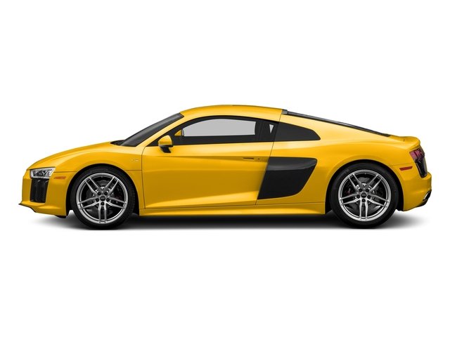
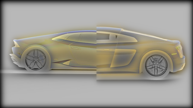
Audi source: https://www.nadaguides.com/Cars/2017/Audi/R8/2-Door-Coupe-Quattro-V10-Plus/Pictures/Print
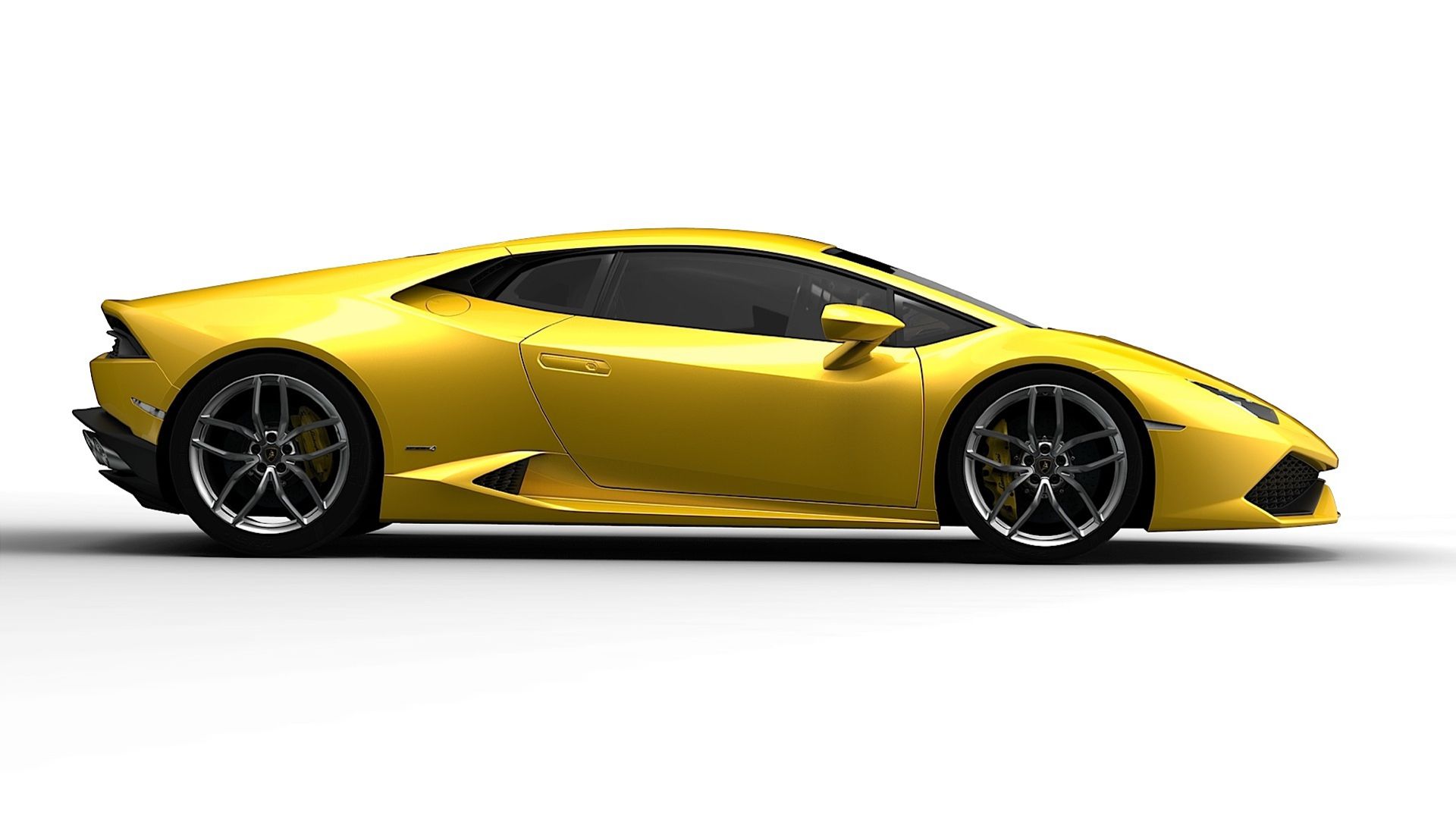
Lambo source: https://ar.pinterest.com/pin/240661173812710017/?amp_client_id=CLIENT_ID(_)&mweb_unauth_id=%7B%7Bdefault.session%7D%7D&simplified=true
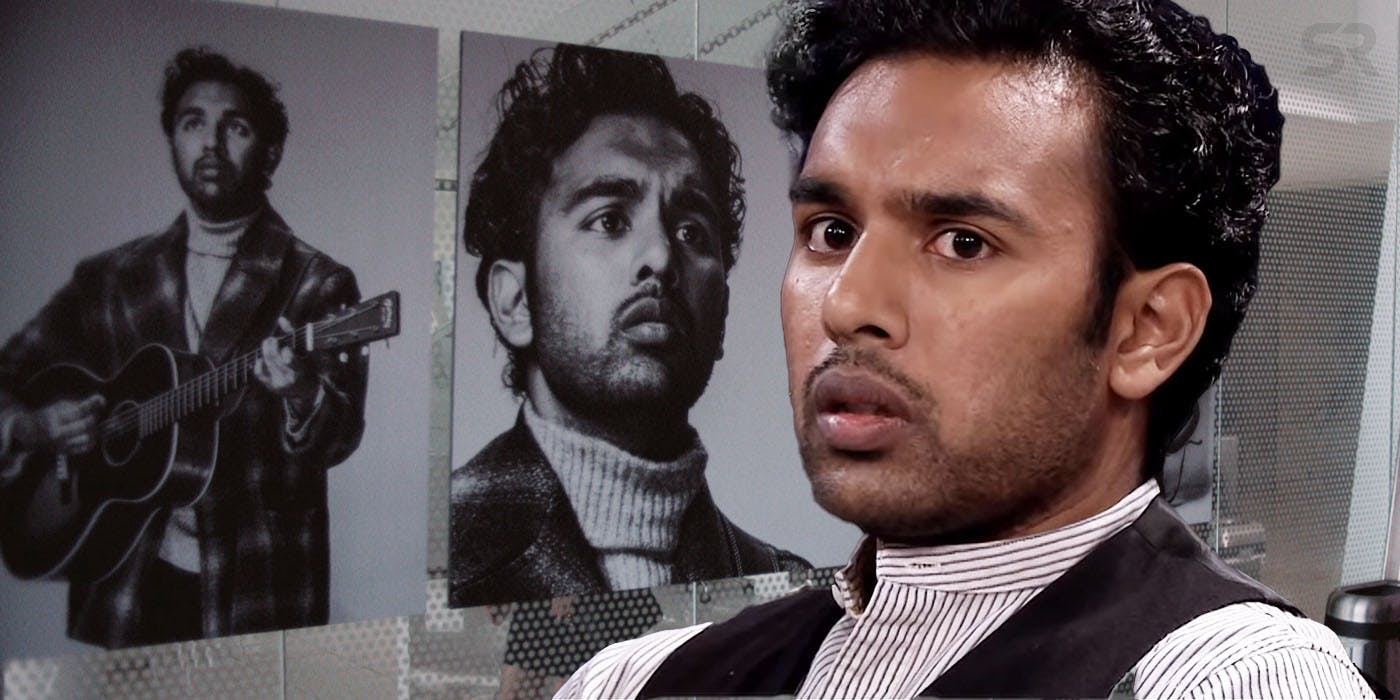
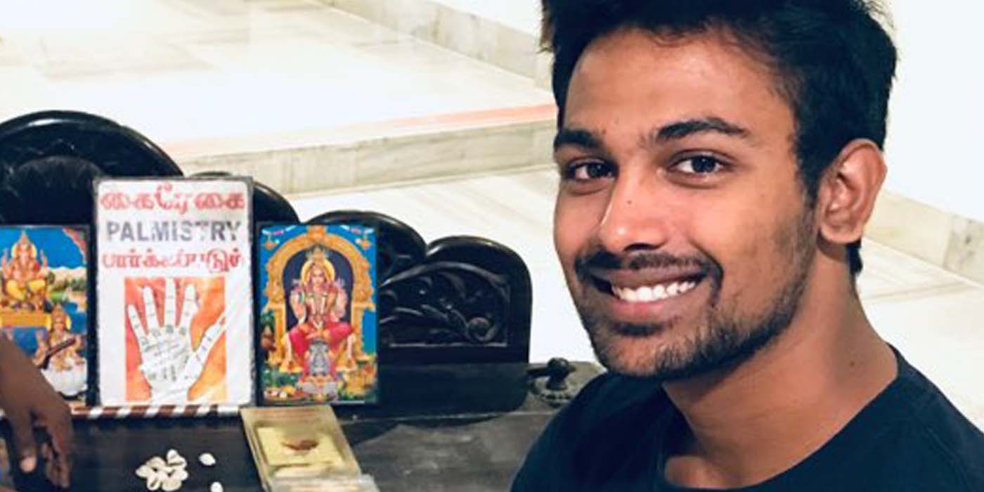
Jack Malik source: https://www.buffalorising.com/2020/08/five-cent-cine-at-home-yesterday/
In this part, we will define a function that constructs Gaussian and Laplacian stacks of images. These will be key to eventually constructing our blended, oraple image in part 2.4. The general approach for constructing the Gaussian stack was by simply convolving the original image with a 2D Gaussian (i.e. running a low_pass_filter) repeatedly until we reached our stack size, just like with the portrait photo of the lady in the lecture slides (see pyramids function in hybrid_image.py for implementation). And to get the Laplacian stack, which is simply the bands of high frequencies in between the images of the Gaussian stack, all we have to do at each level is take our current Gaussian and subtract the Gaussian one level "before" (less blurry) than it. Upon scaling this image to fit in our desired range [0, 1], we end up with a depiction of the high frequencies as our Laplacian (see pyramids function in hybrid_image.py for implementation). Acknowledgements to the Burt and Adelson paper on Multiresolution Splines.
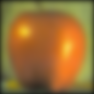
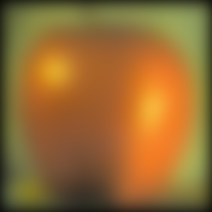
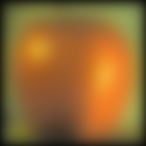
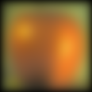


In this part, we use the Gaussian and Laplacian pyramids we built in the last part (along with a spline function that blends them together using a mask, as recommended in page 230 of the Burt, Adelson paper) to blend two images together!
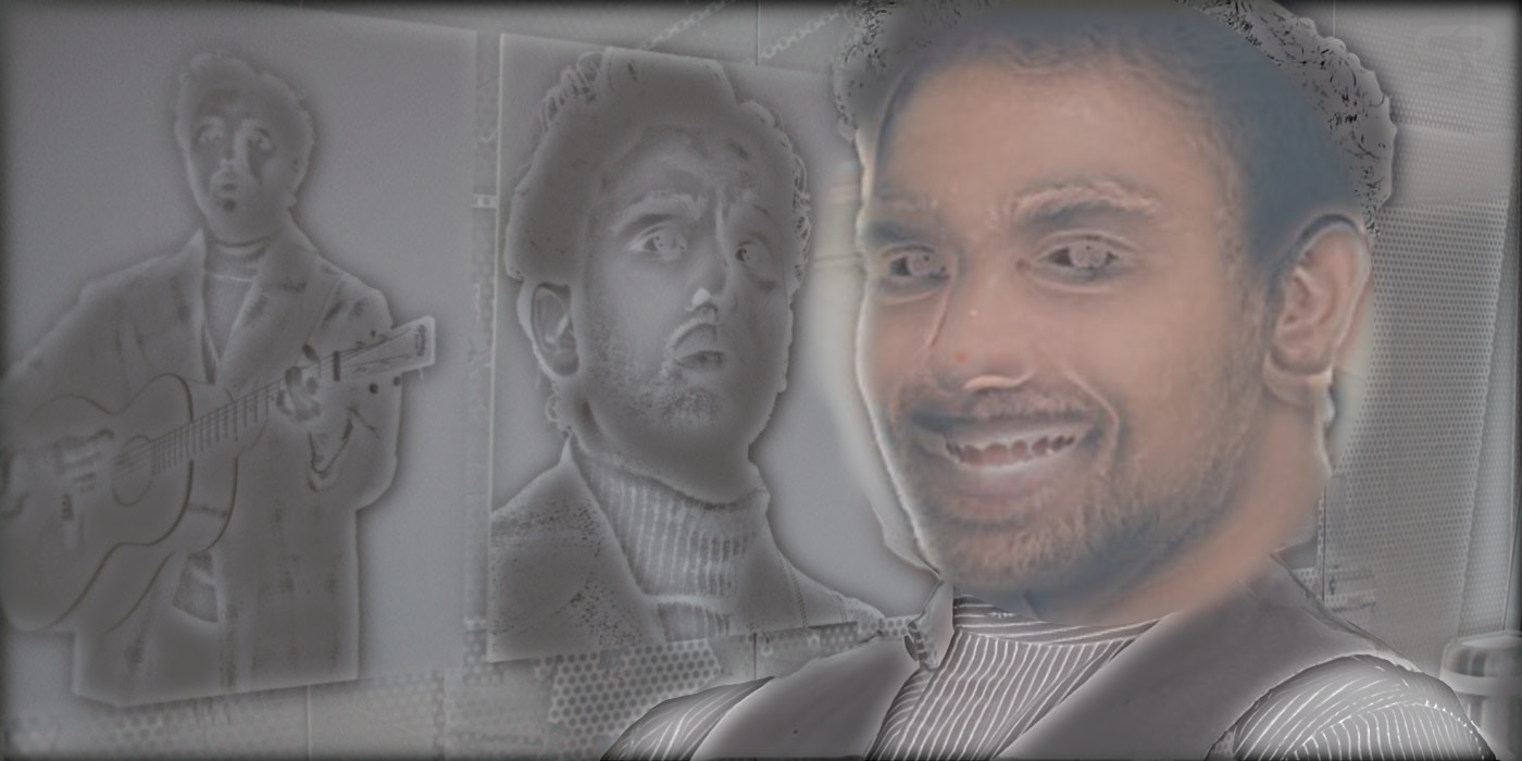
For this next one, I had to use an irregular mask to blend the images together. I'd been told I looked like Jack Malik from Yesterday, so I figured why not see if I can blend myself onto his face of course.

The most valuable thing I learned from this project was developing an intuition for thinking about images in terms of frequencies, both just from looking at an image and thinking about what a high-frequency contour (e.g. from taking partials of it) may look like and visualizing / analyzing it in the Fourier space.