CS 194-26: Intro to Computer Vision and Computational Photography,
Fall 2021
Project 2: Fun with Filters and Frequencies
Hamza Mohammed
Project Overview
The aim of this project is to explore the effects of implementing
filters and frequency blending on an image to manipulate it in various
ways. In part 1, this involves adding convolutions for edge detection.
Part 2 deals with image sharpening, as well as the forming of hybrid and
blended images via the combination of blurred and sharpening images,
visualized by their Fourier transformation graphs. The final subpart of
part 2 deals with multi-resolution blending derived by the combination
of blurred images and a mask.
Part 1
1.1: Finite Difference Operator
|
The images below show the original cameraman image, followed
by the resultant image after convolving with finite difference
filters Dx and Dy individually. The
magnitude of the gradience image is derived by applying the
filters for x and y separately, then squaring the resultant
images per pixel, and taking the square root of the sum of the
squared pixel values of both images. The resultant image is the
gradient magnitude image. To form the edge detection image, we
binarize the image to only values of 0 or 1, based on a
threshold pixel value of 0.25, determined qualitatively, to
create a binary edge image (Figure 6).
|
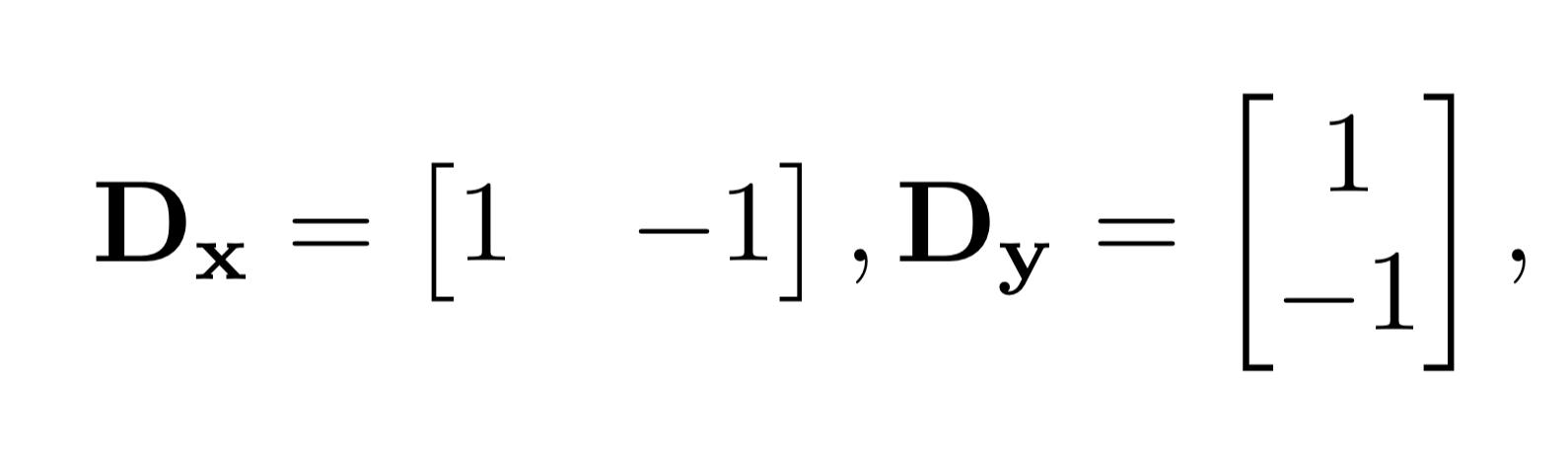
Figure 1: The
finite difference operators Dx and Dy.
|
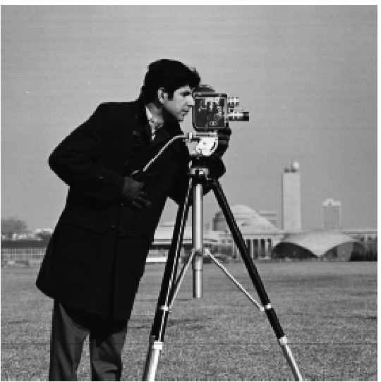
Figure 2:
Original pristine cameraman image.
|
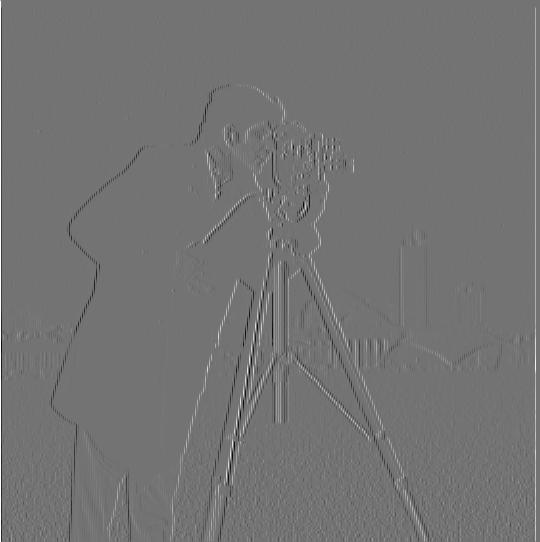
Figure 3:
Horizontal edge detection (convolution with Dx).
|
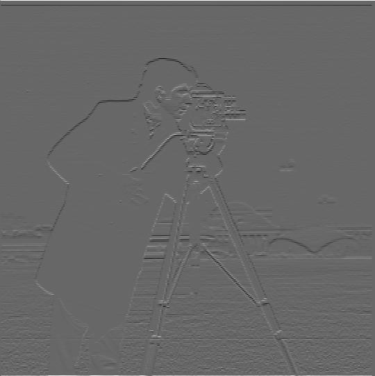
Figure 4:
Vertical edge detection (convolution with Dy).
|
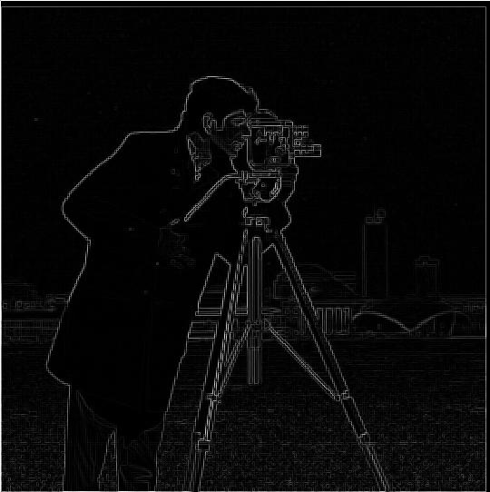
Figure 5:
Horizontal and Vertical edge detection, gradient magnitude
image.
|
1.2: Derivative of Gaussian (DoG) Filter
As seen in Figure 6, there still exist a significant amount of noise
in the image, despite the threshold values, such as in the grass field.
To avoid such noise, we can introduce blurring. We add gaussian blur to
the image prior to convolving with the finite difference filters
Dx and Dy. After which, we compute the magnitude
of gradient image in the same manner as earlier, albeit now with a
threshold value of 0.07 (Figure 7). The lower value is because the
blurring helps eliminate much of the noise that would be present in the
gradient image, thereby, the threshold need not be so severe. As seen in
the figures below, the image does not have nearly as much noise, e.g.,
in the grass field.
Moreover, convolving the Dx and
Dy
filters with gaussian blur, and then convolving the resulting filter
with the pristine image yielded the same output edge image as applying
the convolutions on the pristine image separately (i.e., the process is
commutative, Figure 8).
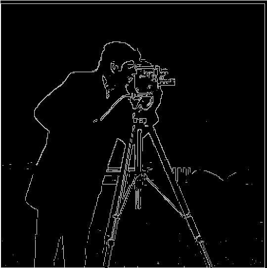
Figure 6:
Image edge map, i.e. Binarized gradient magnitude image with
threshold value 0.25.
|
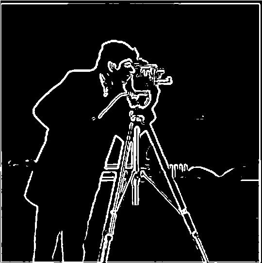
Figure 7:
Image edge map output after applying gaussian blur to image
before edge detection.
|
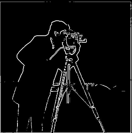
Figure 8:
Image edge map from applying gaussian to Dx and Dy for a
derivative of gaussian filters. Edge detection via single
convolution.
|
Part 2
2.1: Image Sharpening
The process of image sharpening was done using the unsharp masking
technique. This process uses the same gaussian filter to blur the image
and subtracts this blurred image from the original image. This
difference matrix of pixels essentially contains the “sharp” components
or high frequencies of the image. E.g., Building edges for taj mahal,
the fur of the cat, or the edges of the clouds and ripples in the water
for the golden gate image, (Figures 11, 16). By adding the difference
matrix of pixels back to the original image, we amplify these high
frequencies, thereby creating a “sharper” image (Figures 12, 13, 17-23).
As shown in the figures below, the range of high frequencies
that are amplified, determined by the alpha and sigma values of the
gaussian matrix used to blur the image, determine how sharpened the
image look. With alpha=11, sigma=5, the sharpened images amplify edges
such as cat fur, edges of the building or clouds, or the waves in the
water, to a much greater extent, than with alpha=5 and sigma=2. In other
words, increasing the gaussian kernel causes the "edges" and other
"sharp features" of the image to overwhelm the rest of the elements
within the image following amplification (Figures 12 vs. 13, 17 vs. 18,
& 19-23).

Figure 9:
Original Taj Mahal image.

Figure 10: Taj
Mahal after applying gaussian blur.
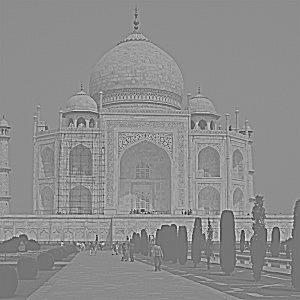
Figure 11: High
frequency mask of Taj Mahal (original image - gaussian blur
image).
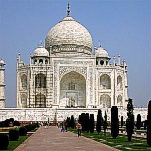
Figure 12:
Sharpened Taj Mahal image with alpha=5 and sigma=2 for the
gaussian filter kernel used to blur.
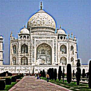
Figure 13:
Sharpened Taj Mahal image with alpha=11 and sigma=5 for the
gaussian filter kernel used to blur.

Figure 14:
Original image of golden gate bridge.
Source:
https://www.istockphoto.com/photo/golden-gate-bridge-gm472318236-63302645

Figure 15:
Golden gate bridge after applying gaussian blur.
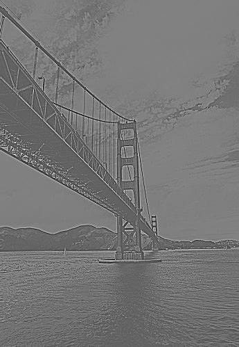
Figure 16: High
frequency mask of golden gate bridge (original image - gaussian
blur image)..
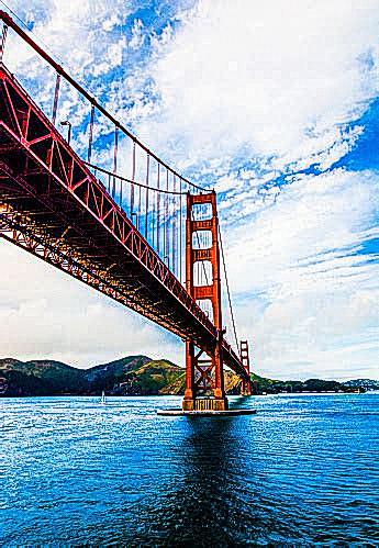
Figure 17:
Sharpened golden gate bridge image with alpha=5 and sigma=2 for
the gaussian filter kernel used to blur.
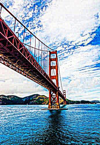
Figure 18:
Sharpened golden gate bridge image with alpha=11 and sigma=5 for
the gaussian filter kernel used to blur.

Figure 19:
Original image of kitten.
Source: Kitten searched on Google
Images
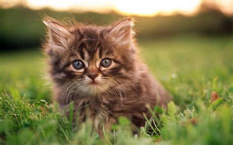
Figure 20:
Sharpened image of kitten using gaussian kernel with alpha 2,
sigma 1 for blurring to generate high frequency mask.
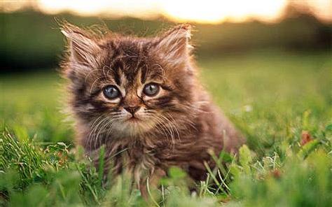
Figure 21:
Sharpened image of kitten using gaussian kernel with alpha 4,
sigma 1 for blurring to generate high frequency mask.

Figure 22:
Sharpened image of kitten using gaussian kernel with alpha 5,
sigma 2 for blurring to generate high frequency mask.
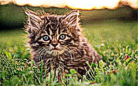
Figure 23:
Sharpened image of kitten using gaussian kernel with alpha 11,
sigma 5 for blurring to generate high frequency mask.
Moreover, although we can sharpen an image, if we artificially blur
an image via gaussian blurring, and try to restore the original image
using our technique, the resultant image is still blurry. The
resharpened image only restores the high frequencies, but the data
lost in the blurring (i.e., low frequencies such as the details on the
walls of the taj mahal) is not restored. This indicates that the
unsharp masking technique does not introduce any new information into
the image.

Figure 24:
Blurred Taj Mahal image. (gaussian with alpha=9, sigma=4).
|

Figure 25:
Resharpened Taj Mahal image.
|
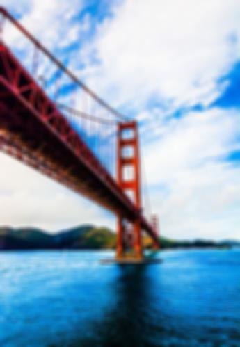
Figure 26:
Blurred golden gate bridge image. (gaussian with alpha=9,
sigma=4)..
|

Figure 27:
Resharpened golden gate image.
|

Figure 28:
Blurred kitten image. (gaussian with alpha=9, sigma=4).
|

Figure 29:
Resharpened kitten image.
|
2.2: Hybrid Images
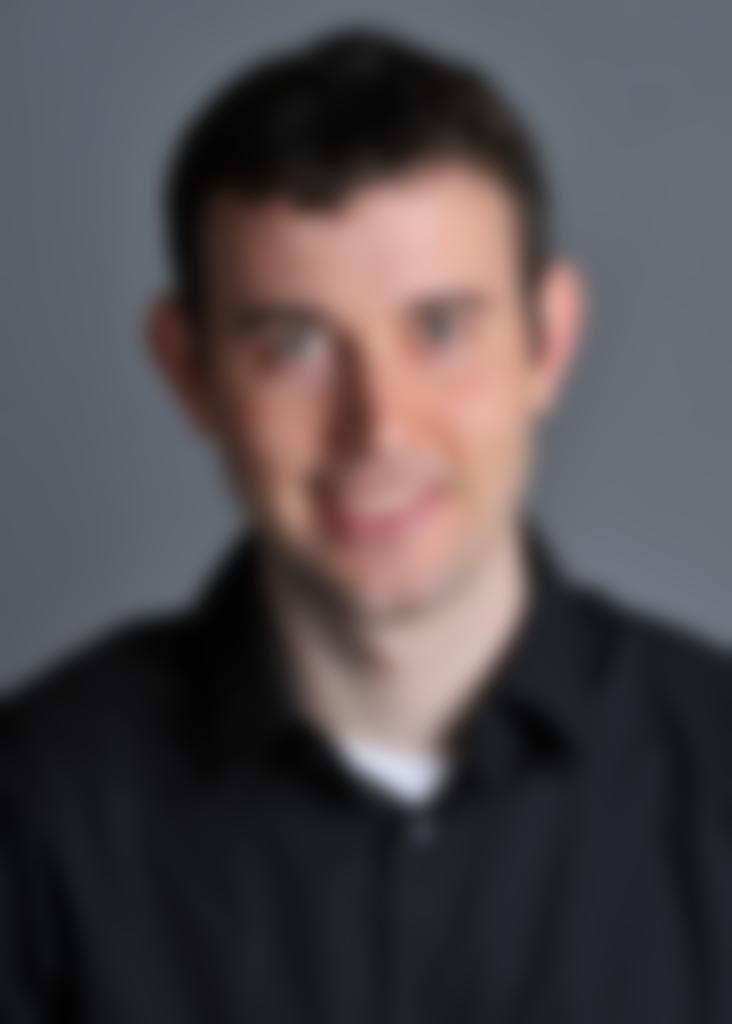
As seen from the unmask sharpening technique, gaussian blurring of
an image is effectively a low-pass filter. In this manner, a series of
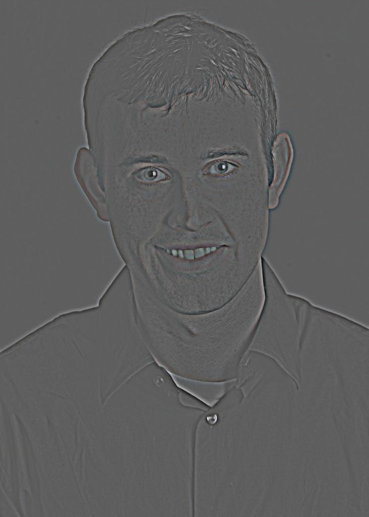
hybrid images were constructed by combining the high frequencies of
one image with the low frequencies of another. The high frequency
image was constructed by subtracting the gaussian blur image from its
original image, while the low frequency image was constructed by
applying the gaussian filter. The combined hybrid image is intended on
looking like the high-frequency image when close up due to the detail
that is maintained within it, and the low frequency image from farther
away.
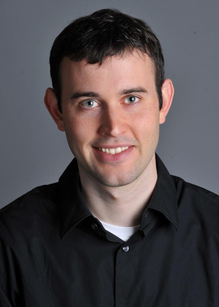
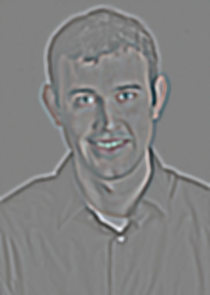
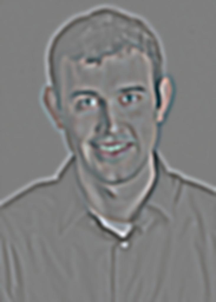
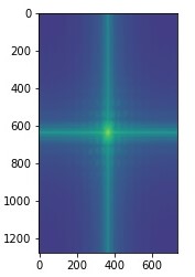
This is best illustrated with the Einstein Monroe
hybrid image, or the Derek Nutmeg hybrid image.
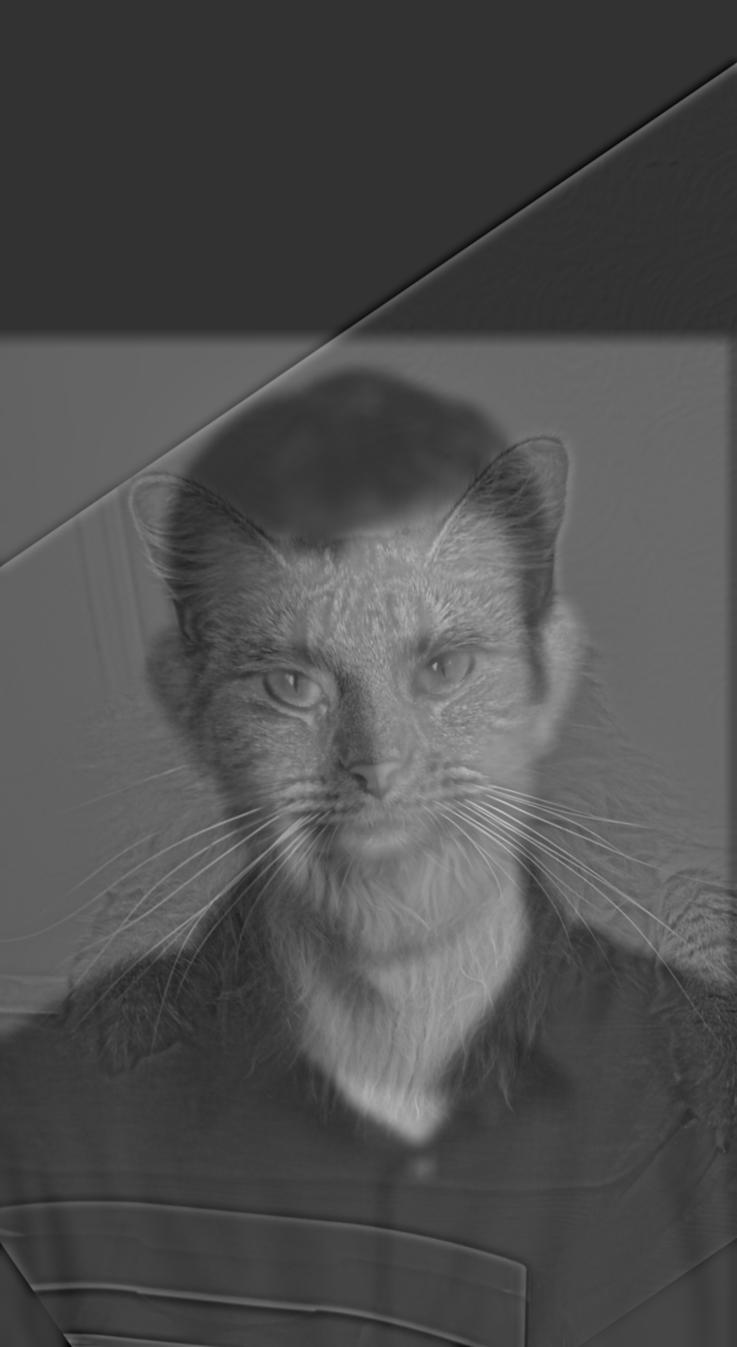
Figure
30: Hybrid Image of Derek (low frequencies) and Nutmeg (high
frequencies).
|
Figure
31: Frequency spectrum of original Derek image.
|
Figure
32: Frequency spectrum of original Nutmeg image.
|
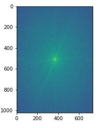
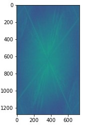
Figure
33: Frequency spectrum of low-pass filtered Derek image. The
high frequencies depicted in the corners of the graph are
absent in comparison to the original image.
|
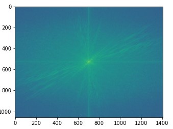
Figure
34: Frequency spectrum of high-pass filtered Nutmeg image.
The high frequencies of the image are intensified in
comparison to low-frequencies compared to the original
image.
|
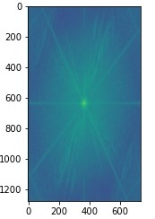
Figure
35: Frequency spectrum of the hybrid Derek and Nutmeg image
from Figure 30. Hybrid image has frequencies in both low and
high range unlike the two filtered images used to construct
the hybrid image.
|
Some Additional Examples of Hybrid Images
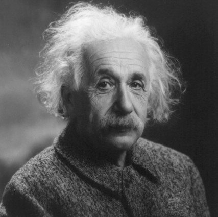
Figure
36: Original image, Einstein.
Source:
https://openlysecular.org/freethinker/albert-einstein/
|
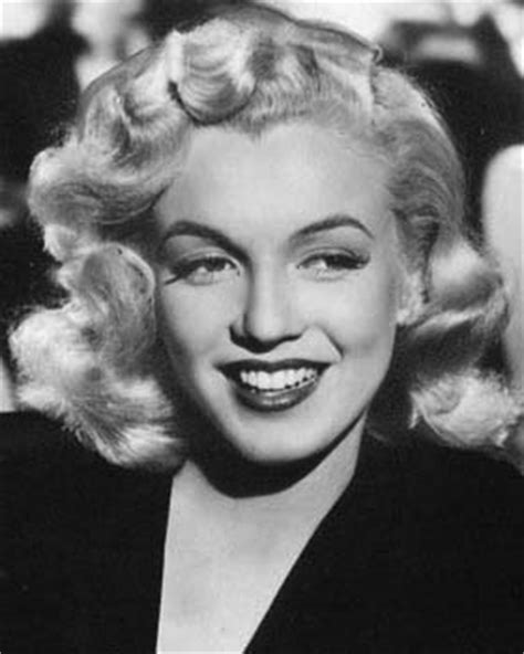
Figure
37: Original image Monroe.
Source:
http://projects.latimes.com/hollywood
/star-walk/marilyn-monroe/
|
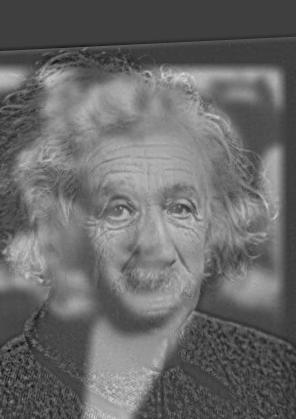
Figure
38: Hybrid image of Einstein (High Frequencies), and Monroe
(Low Frequencies).
|
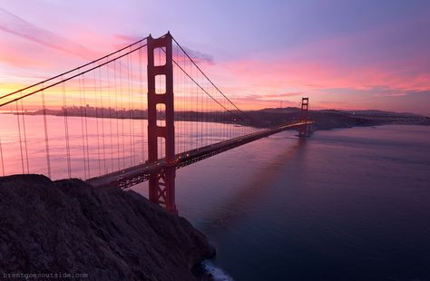
Figure
39: Original image, Golden Gate Bridge in the morning.
Source:
https://www.pinterest.com/
pin/473370610807573298/
|
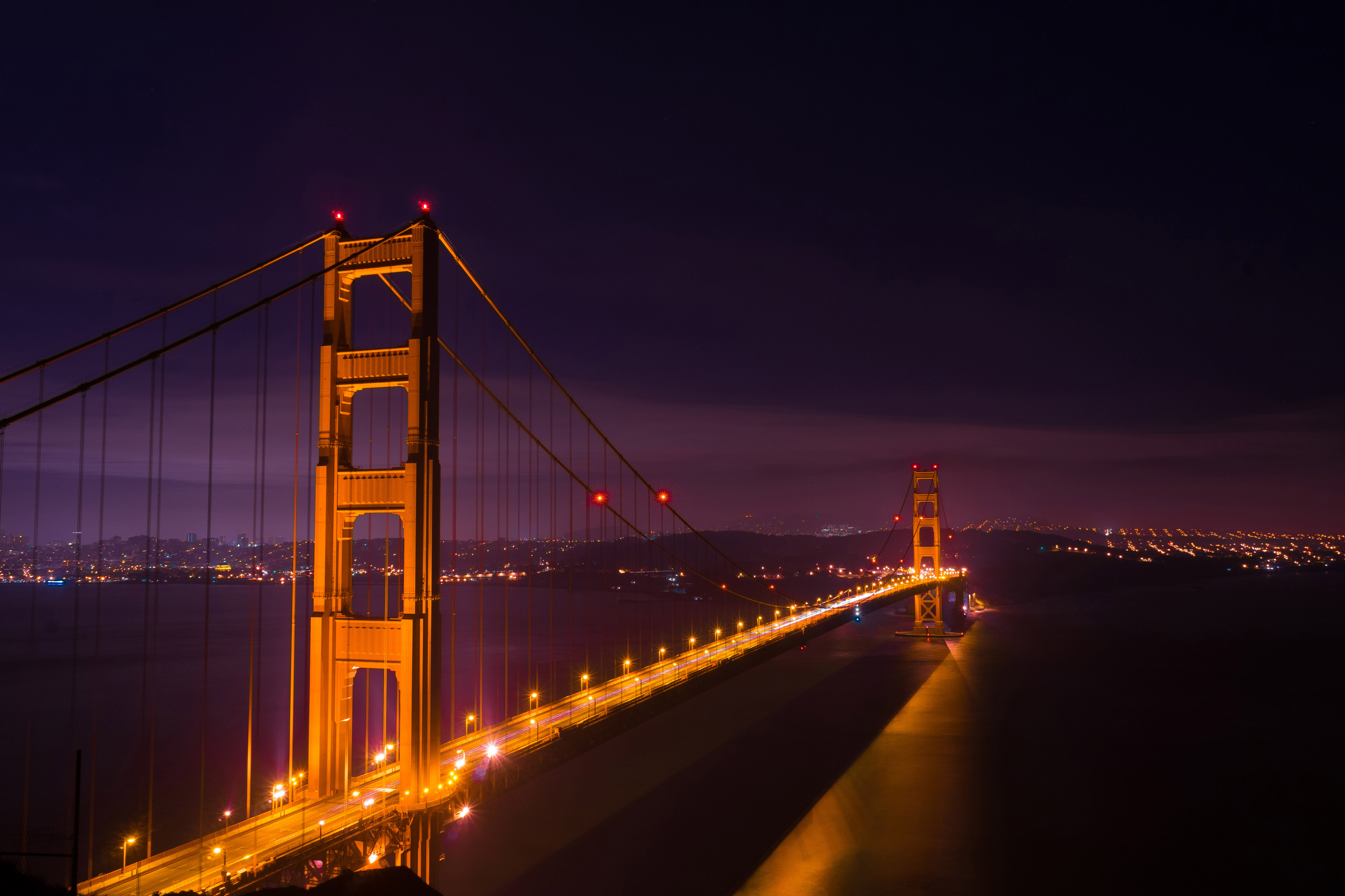
Figure
40: Original image, Golden Gate Bridge in the night.
Source:
https://www.goodfreephotos.com/united-states/california/san-francisco/golden-gate-bridge-at-night-in-san-francisco-california.jpg.php
|
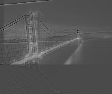
Figure
41: Hybrid image of the Bridge in the morning (High
Frequencies), and night (Low Frequencies). Keeps the detail
of the bridge and scenery from the morning, and combines it
with the lights of the bridge and traffic from the
night.
|
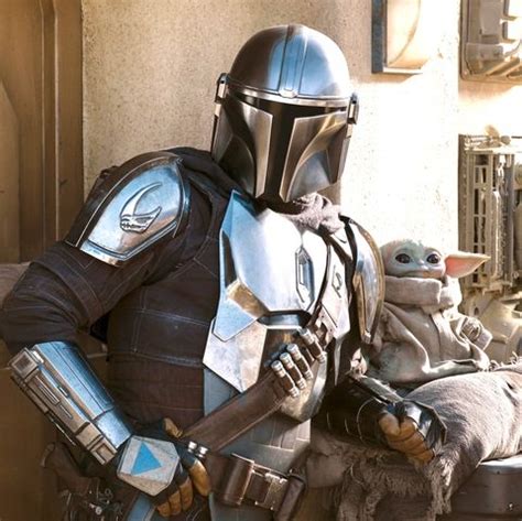
Figure
42: Original image, Mando from Star Wars.
Source:
https://www.menshealth.com/entertainment/a34891653/mandalorian-season-3-cast-release-date-trailer/
|
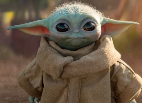
Figure
43: Original image, Baby Yoda from Star Wars.
Source:
https://www.indiatoday.in/trending-news/story/california-wildfires-kitten-resembling-baby-yoda-rescued-by-firefighters-read-post-here-1725608-2020-09-26
|
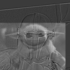
Figure
44: Hybrid image of Mando (High Frequencies) and Baby Yoda
(Low Frequencies). Aim was to make a hybrid image with
Mando's helmet to give the appearance that baby yoda was
wearing Mando's helmet. However this doesn't seem to work as
it only appears we simply stacked Mando's image on top of
baby yoda's image without creating a "hybrid" image. It
seems that combining images that don't already have some
similarity, e.g two faces, or two bridges is difficult as
the frequcnies of the image vary too much for their
combination to be a realisitc hybrid image.
|
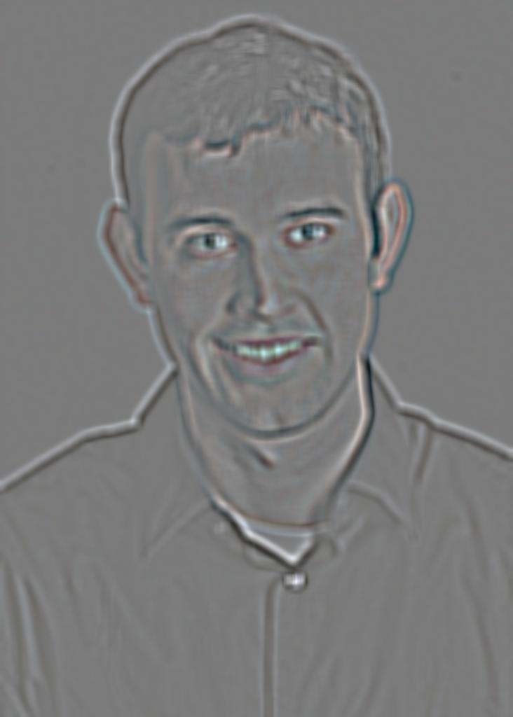
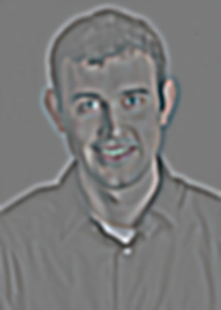
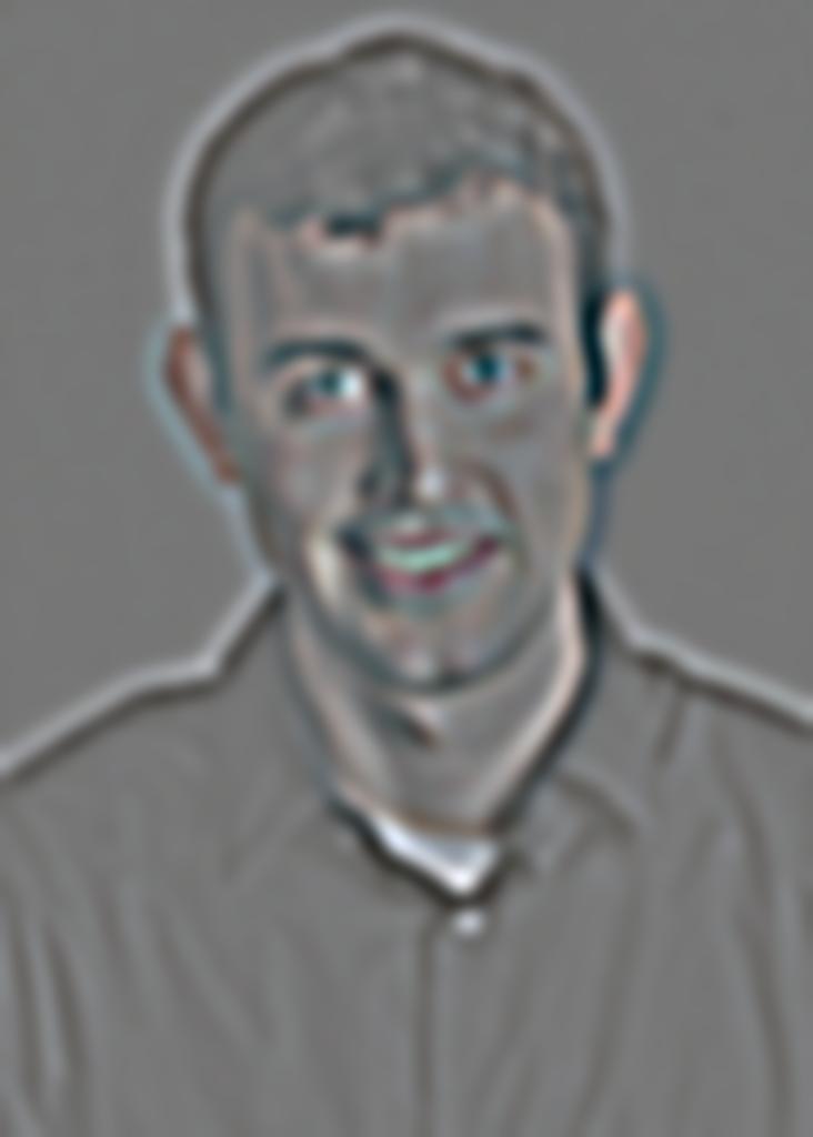
2.3: Gaussian and Laplacian Stacks
To implement more complex types of blending, the Gaussian and
Laplacian stacks were generates for the images to be blended together.
The Gaussian stack contains the same image but with increasing levels
of Gaussian blurring, while the Laplacian stack contains the same
image but with increasing levels of Laplacian sharpening. Here
Laplacian sharpening at ith level is calculated by
subtracting the original image with the gaussian blurring at level
i-1. Thereby, the Laplacian stack contains the same image but filtered
for varying ranges of frequencies, higher and higher per level. i.e.,
edges of the image at varying blur levels.
Figure 45: Gaussian
stack of Derek image with increasing level of guassian blur as levels
increase from left to right in stack
Figure 46: Laplacian
stack of Derek image with increasing level of laplacian sharpening as
levels increase from left to right in stack. At each level we can see
a different range frequency represented from the original image.
The Orapple Stack
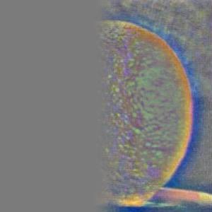
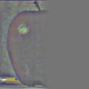
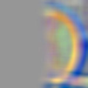
Figure 47.1:
Laplacian stacks for the orapple where the first column is the apple
stack, the second column is the orange stack, and the third is their
combination stack. The images represent the high to low frequencies of
the original and combination (Figure 48) images as row index increases
which corresponds with increasing stack level
Figure 47.2:
Guassian stack of mask used to create the orapple via multi-resolution
blending. The mask has a vertical seam and is originally a binarized
image. Guassian kernel uses alpha=40, sigma=20.
2.4: Multi-Resolution Blending
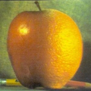
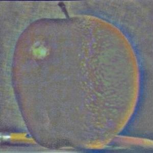
Figure 48: The
Orapple! Combination image from blending two images using their
laplacian stacks (part 2.4).
Multi-Resolution blending is the process of blending two images
using their Laplacian stacks generated via the algorithms developed in
part 2.3. The process uses a mask for whom a gaussian stack is
generated also from part 2.3. This allows one to create a function
that smoothly blends the transition between the two images along the
seam of a mask. The mask is a binarized pixel matrix (black and white
image) with pixel values of 0 or 1.
The algorithm implemented for multi-resolution blending was as
follows:
At each level of the stack, create the linear combination pixel matrix
of the corresponding Laplacian images from the stack based on the
pixel values from the gaussian blurred mask for that level. Add all of
these linear combinations together to get the multi-resolution blended
image (refer to Figure 47 and 48, to see this process applied to
recreate the Orapple).
Below are some additional examples of blended images. Note the
inclusion of color in the blended images, implemented by conducting
the blending procedure along all 3 channels of both images separately,
and stacking together the blended channels to output a colorized
blended image
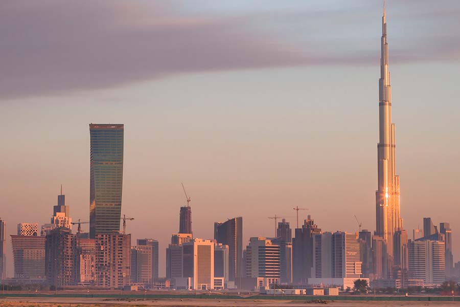
Figure 49:
Original image, Burj Khalifa.
Source:
https://www.worldfortravel.com/the-impressive-burj-khalifa-dubai-uae/
|
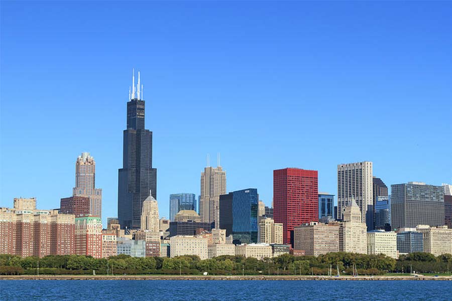
Figure 50:
Original image Chicago skyline.
Source:
https://photos.com/featured/3-chicago-skyline-fraser-hall.html
|

Figure 51:
Mask used to blend the two images. Aim was to add the Burk
Khalifa to the Chicago skyline.
|
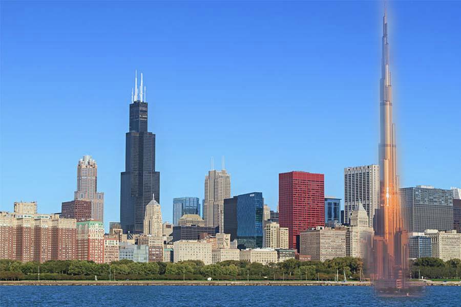
Figure 52:
Resultant blended image, adding Burk Khalifa to Chicago skyline.
Unfortunately, the images are not color balanced with respect to each
other, as it was difficult to find images of both the Chicago and
Dubai skyline that were at approximately the same angle. Moreover,
because of the sharp edges within both images, and how the mask is the
outline of the Burj Khalifa, the building ends up having softened
edges. Using a lower kernel size for the Gaussian would reduce this
effect at the cost of a significant loss in color, but with a tighter
seam. As a result, the building has a glowing appearance from the
softening of its edges along the seam of the mask.
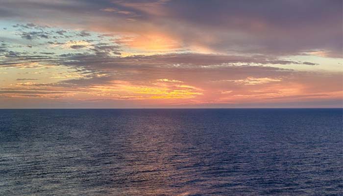
Left: Figure 53: Original image, ocean view in the morning.
Source:
https://ocean.si.edu/ocean-life/sharks-rays/whats-ocean-worthin-dollars
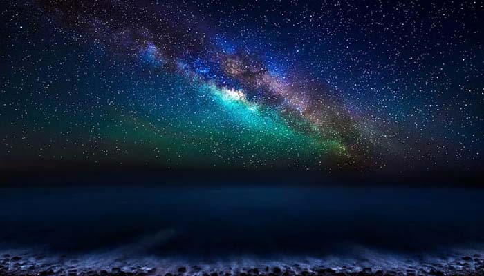
Middle: Figure 54: Original image, ocean view in the night.
Source:
https://www.wallpaperflare.com/milky-way-galaxy-from-the-canary-islands-ocean-sky-night-stars-wallpaper-uvace
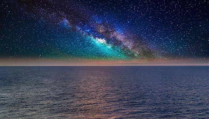
Right: Figure 55: Resultant blended image. The mask was a
simple horizontal seam that blended along the horizon of the two
images, with ocean in the morning being at the bottom, and ocean in
the night at the top. This led to a very nicely blended image with a
clear view of the ocean with its waves from the morning, and the
starry night sky from the ocean view in the night. This blended
image turned out better than I thought most likely because of how
well aligned the two images were, and the simplicity of the masking
needed to blend them together.
Armed with this new blending technqiue, let's re-attempt combining
Baby Yoda with Mando. The goal is to create a blended image with baby
yoda wearing Mando's helmet.
First let's choose more optimized source images such that both
charecters' faces are in frame at the same angle.
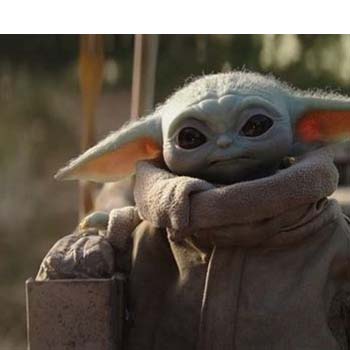
Figure 56:
Original image, Baby Yoda.
Source:
https://thelakelander.com/baby-yoda-is-here-to-save-us-all/
|
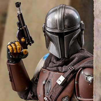
Figure 57:
Original image, Mando.
Source:
https://www.sideshow.com/whats-new/the-mandalorian-sixth-scale-figure-by-hot-toys/
|
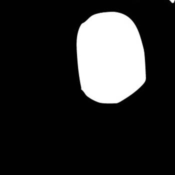
Figure 58:
Mask used to blend the two images.
|
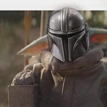
Figure 59:
Blended Baby Yoda image with Mando.
|
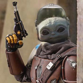
Figure 60:
Blended Baby Yoda image with Mando, but image ordering is
reversed.
|
As seen in figure 59, multi-resolution blending is far more
successful at blending Baby Yoda with Mando such that it appears
Baby Yoda is wearing Mando’s helmet. With the appropriate mask, the
blending was almost perfect! Of course, we would still have to do
something with Baby Yoda’s ears which poke out and decrease the
realism of the blended image. Also, there is a white bar on the top
of the blended image. This is because Baby Yoda’s reference image
had to be cropped to properly align with Mando’s helmet. This
represents a possible extension for part 4, which is the
implementation of an alignment algorithm, such as the one used in
part 2.2. Albeit this doesn’t solve the issue of the white bar. We
would likely have to find another reference image that is better
aligned with Mando’s image, or include Deep learning algorithms,
such as ImageGPT from OpenAI to “fill in” any such white/blank
spaces following an alignment procedure.
Moreover, despite the significant improvement in the
blended image in comparison to the hybrid version, like with figure
52, there still exists some softening along the edges of the helmet
which corresponds with the seams of the mask.
Just for fun, I also tried reversing the images to make it
look like Baby Yoda was in Mando’s suit (Figure 60). Not nearly as
realistic, but just as funny, cuz this is the way. (sorry, but I had to say it)
What I Learned
This project got progressively more interesting. By far, part 4 was
the most interesting and fun. By carefully choosing the appropriate
source images, a good mask, along with optimized gaussian kernel, you
could get achieve very nice image blends (e.g., figure 55 or 59). I
learned this was through the linear combination of the Laplacian stacks
of the source images whose weights are determined by a gaussian blurred
mask. The blurring of the mask allowed for a smoother transition between
the images. From experimentation, the best blended image was generated
when the low-frequencies of the images are combined with the weights
from the blurrier levels (higher levels) of the gaussian stack for the
mask, while the high-frequencies of the images are combined with the
weights of the sharper levels (lower levels) of the gaussian stack for
the mask. From lecture and from reading the textbook, I learned this is
because each level of the Laplacian stack deals with a specific spectrum
of frequencies of the two images. Therefore, combining with a variably
blurred mask ensures that low frequencies or combined with greater
overlap across the transition boundary of the mask for a smother blend,
while higher frequencies, that deal with the more detailed edges of the
images, are combined with much less overlap to give the appearance of a
sharper transition of the edges/details within the images (i.e.,
maintaining their separation within the blended image). I never realized
the significance of the frequency spectrum of an image, especially with
regards to image manipulation and comprehension.
I wasn’t surprised when
I found out that an extensive number of deep learning techniques use or
manipulate the frequency spectrum of an image for computer vision
applications.