|
|
In this project, I implemented face morphing (blending together both the shape and appearence of people's faces).
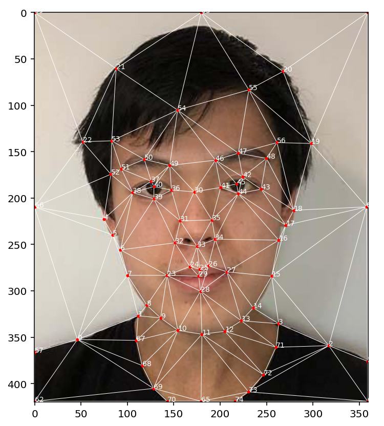
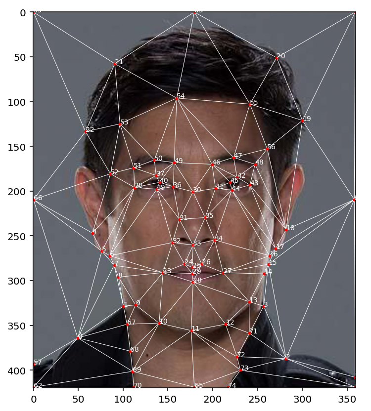
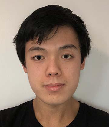
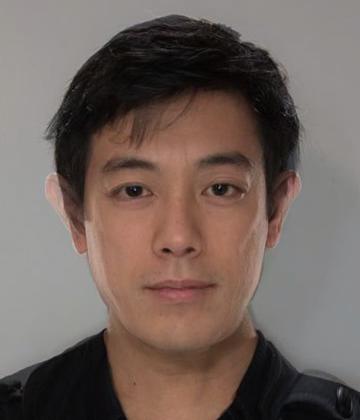
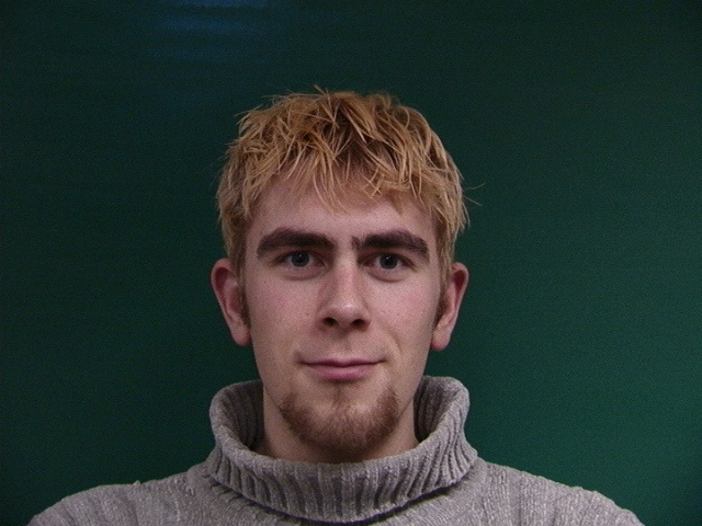
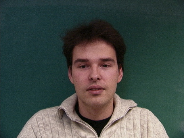
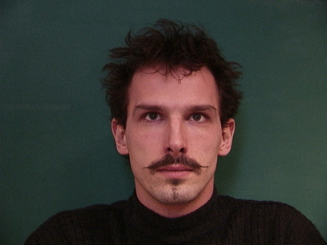
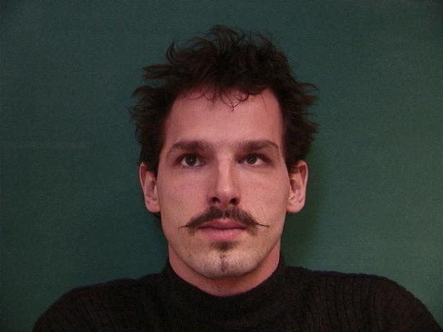
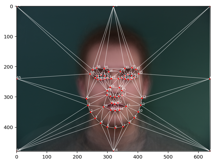
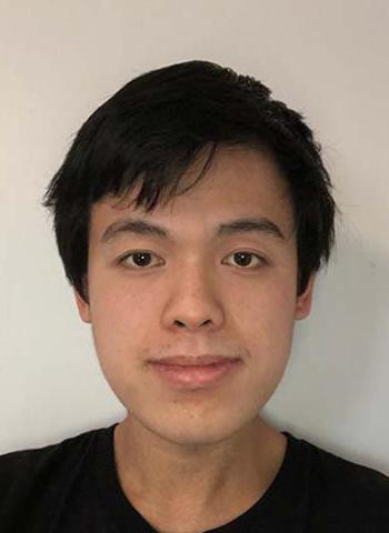
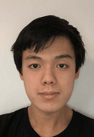
For the first part of this project, I blended my face with Grant Imahara (source). The first step of the morph is to define matching keypoints on both faces. I used ginput in python to create a interactive tool for adding the points. Using the points, I created a Delaunay triangulation using scipy based on the points at the midway shape (to minimize distortion).
|
|
|
I had a total of 75 carefully chosen points on each face (this took a long time to get right). In addition to the features of the face, I also added points along the border of the image, along the sides and neckline of the shirt, and along the hairline. Once challenge of morphing to Grant is that his neck is much wider than mine, so I had to make sure that the points I defined along the chin were precisely matched.
I then implemented the code to compute the affine transformation between triangles (using a system of equations and np.linalg.pinv) and bi-linear color interpolation (using interpn) for inverse sampling. At each "midway" triangle, I compute two transformations to the triangles in the source and destination image, sample the pixels using the transform and the interpolation function, and then cross dissolve between the samples.
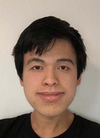
The midway face is created by morphing both faces in to the average shape, and blending their colors equally.
|
|

|
And here is the 45-frame animated morph between the two faces.

The facial features, shirt, neck, and hair all blend realistically, but the left ear isn't perfect because my ears are covered and Grant has large ears (the right ear works surprisingly well though).
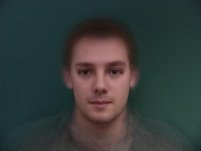
I chose to work with the dataset of the Danes and selected the subpopulation of men with blank expressions.
To compute the average face, I first had to find the average shape (computed from averaging the points of each face) and morph each face to the average shape.
Here are some examples of Danes being morphed to the average male shape.
|
|
|
|
|
|
I calculated the mean of these morphed faces to find the average face of the population.
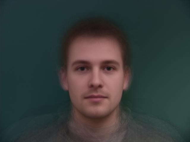 The Average Male Dane
I also tried warping my face to the average geometry, and the average face to my geometry. For my image, I defined a new set of keypoints to match those of the Dane dataset.
|
|
|
|
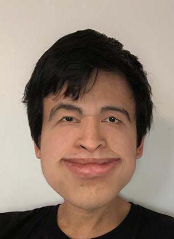
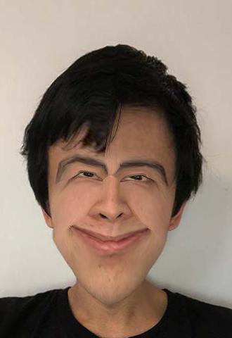
I created a caricature of my face by extrapolating from the population mean of smiling danes with warp_frac = 2. The angled eyes and very large nose/lips are quite extreme.
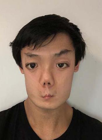
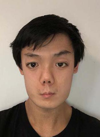
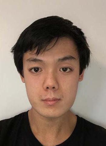
Here's a visualization of me being warped at different amounts from an "anti-smiling-Dane" to a "super-smiling-Dane" (with the warp factor ranging from -1.5 to 1.5).
|
|
|
|
|
|
I also tried creating a smiling caricature by warping myself to a specific Dane's shape, instead of an average. This worked well since I picked a Dane with a large smile, so his features were able to be transferred over more easily. I used warp_frac = 1.5 for this one.
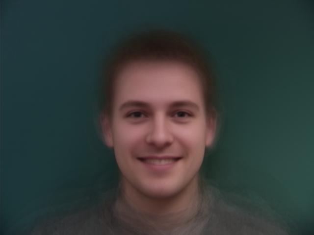
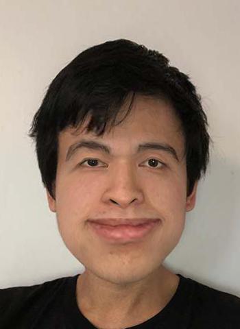
I changed my ethnicity to Danish by morphing myself in to the mean male dane.

|

|

|
I also changed my expression to a smile by morphing myself in to the mean smiling dane.

|
|

|
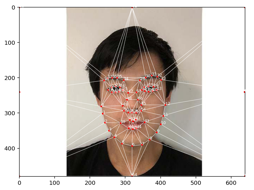
I installed the dlib library and used it for automated detection of face landmarks to be used as keypoints for morphing. I used a pretrained model that has 68 facial keypoints.
The dataset I worked with was headshots of Major League Baseball players, and more specifically SF Giants players. I scraped the images of all players on each team's active roster from the MLB website. In total my dataset had 839 photos.
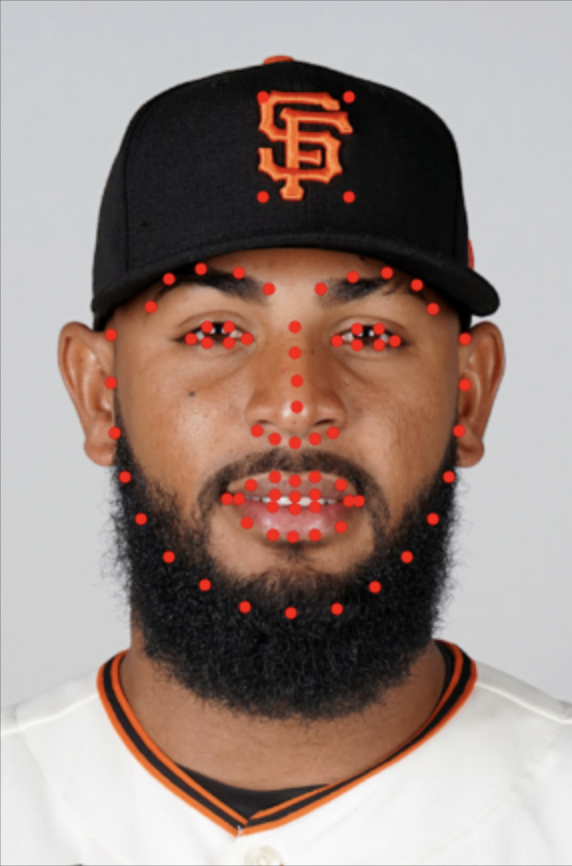
For SF Giants players, I added my own feature detection algorithm to detect the location of the Giants logo on the cap. This is non trivial because the cap also sometimes has a orange button visible at the top of the cap, and a smaller orange logo on the right side of the cap (seen below). To detect the logo, I converted the image to HSV, filtered to only Orange colors, cropped to the upper portion of the image, eroded the image to remove the distractions, and then found the rectangular bounding box of the remaining pixels.
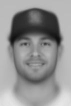
Below is an example of my own feature detection working on the Giants logo, along with the facial keypoints provided by dlib.
Using these keypoints, I created a morph movie that blends together all players on the Giants active roster. Because of the additional keypoints on the logo, the logo moves pretty seamlessly during the morphs. The transition between no smile and smile at 0:11 in the video is my favorite part.
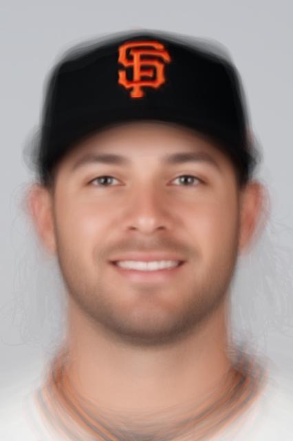
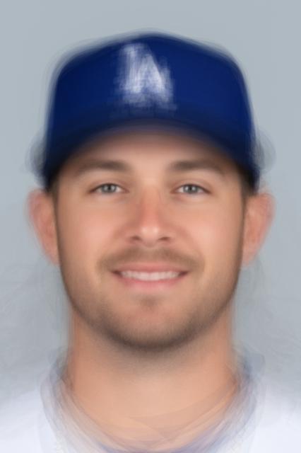
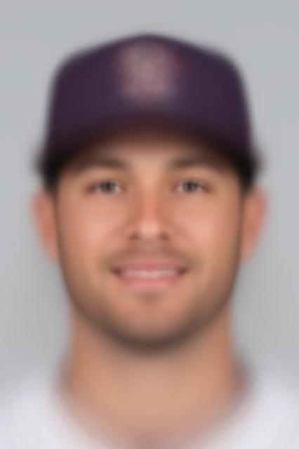
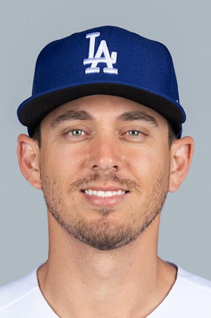
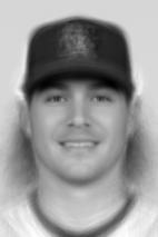
I also calculated the mean image of the Giants, which has a nicely centered logo thanks to the keypoints. I also checked how it compared to other's teams averages, like the LA Dodgers, and the Houston Astros (who have the most number of international players on their roster of any team).
|
|
|
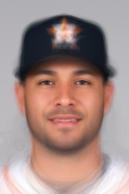
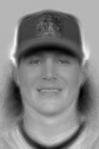
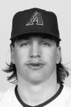
Finally, I morphed the face of all 839 MLB players to the mean shape to find the face of the average baseball player. To spice things up, I also found the player whose appearence was closest to the average face (using the Sum Squared Distance metric from Proj 1). That remarkably average player is Austin Barnes (see how his beard closely aprroximates that of the average?)
|
|
In summary, using automated keypoint detection allowed me to morph and visualize the results for a large dataset very quickly, which would not be possible with tedious manual feature annotation.
Finally, I created a PCA basis on the headshot dataset. The first basis vector (most important) is in the top left corner.
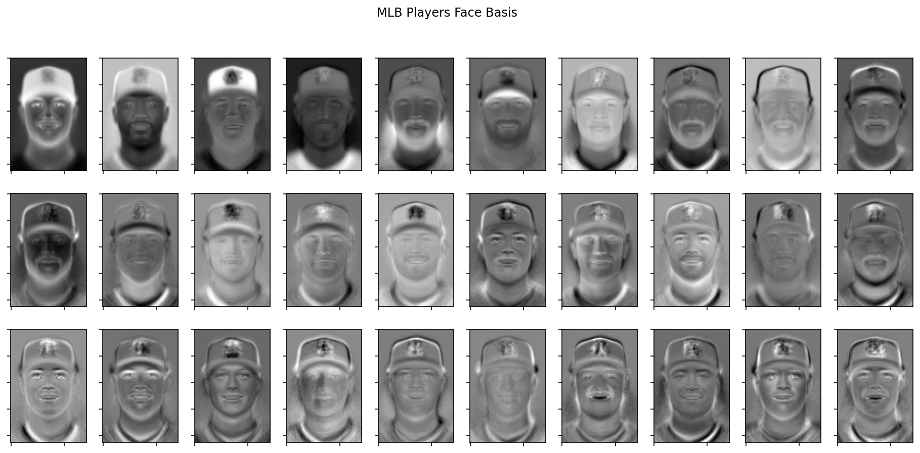
In the first row, you can see some of the facial hair/hairstyle variations. It is also interesting to see the variation in cap logos across the diffferent basis vectors.
I also extrapolated in the PCA basis from the mean to create a caricature image. The low dimension approximation was done with the 25 most important basis vectors.
|
|
|
|
When this player is extrapolated, his long hair grows more prominent since the mean does not have any long hair. This extrapolation is only with the appearence (not the shape) so it is not as exciting as the extrapolation from morphing.