Project 3: Face Morphing

Overview

In this project, we examine faces and try to morph them into each other. In the first part, we define correspondences by hand between two faces and create a triangular mesh out of them. In the second part, we compute a midway face using this mesh. In the third part, we complete a morph sequence between the two faces to watch them seamlessly move into each other. After this, we depart to find the "mean" (average) face of a population (Danish computer scientists). We then use this mean to extrapolate out and create caricatures. And finally, we examine how we can use the fact that faces are a subspace to change the gender of a face.

Part 1: Defining Correspondences

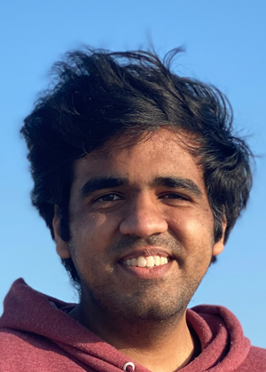
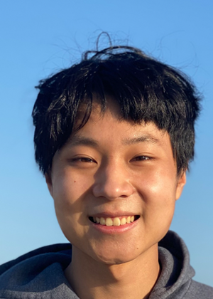
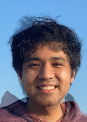
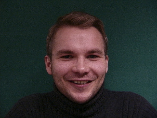
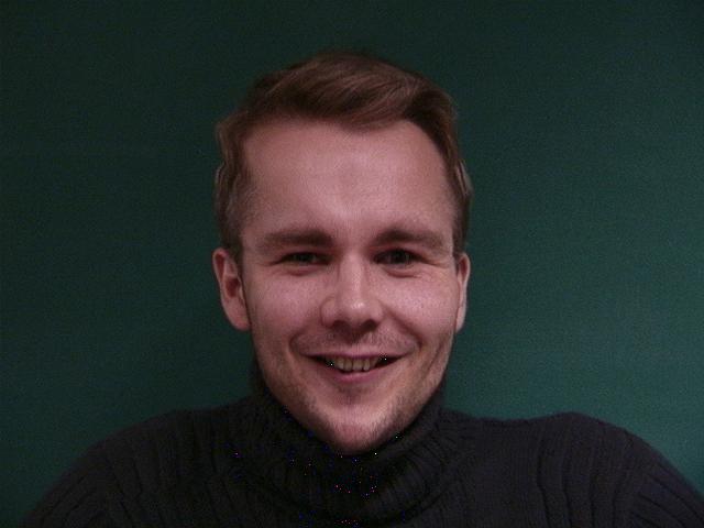
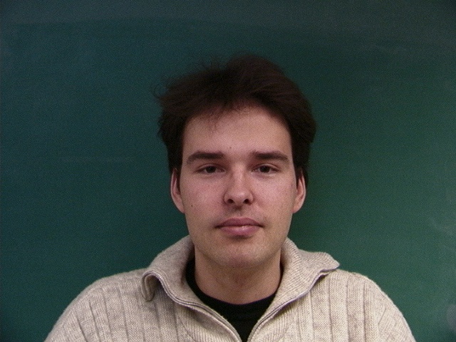
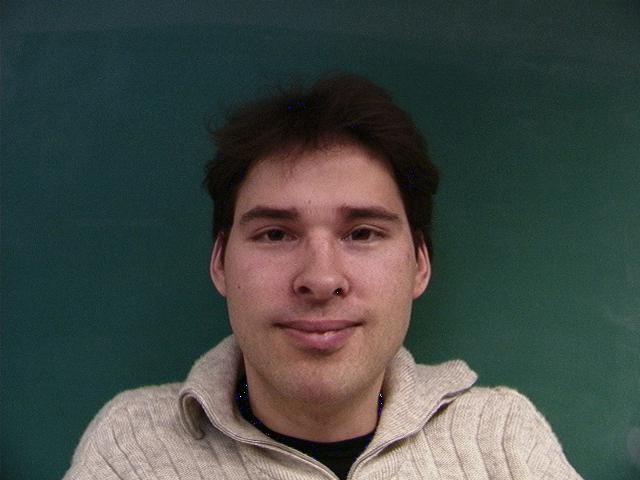
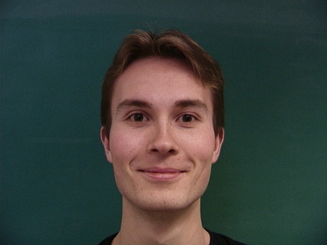
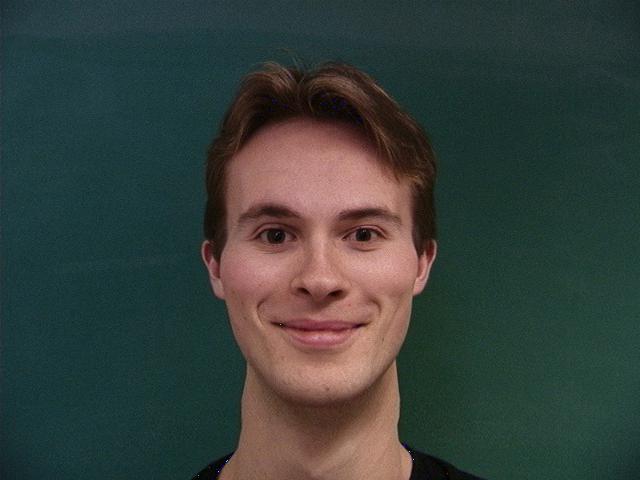
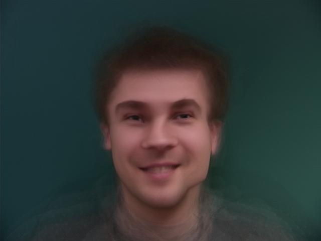
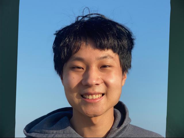
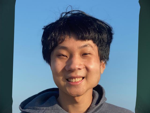
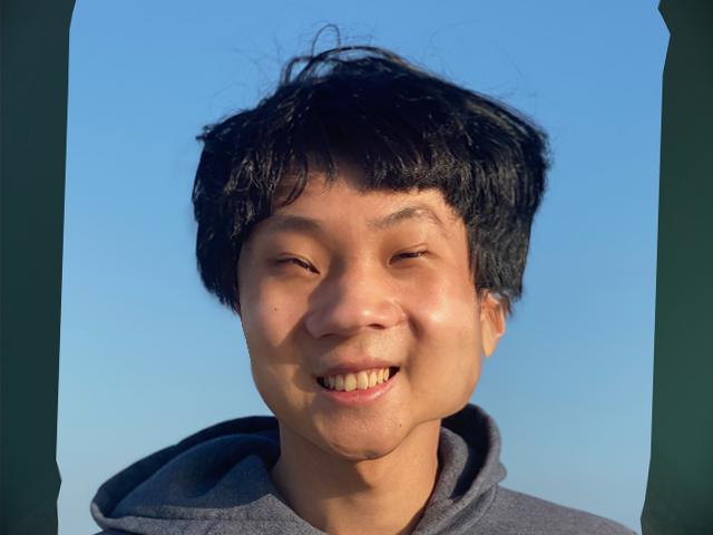
For this part of the project, I was lucky enough to morph together two of my favorite people: my boyfriend Amay, and my best friend Alvin. These photos were taken at a beach in Coronado, CA and provide a consistent background for smooth morphing.

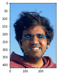
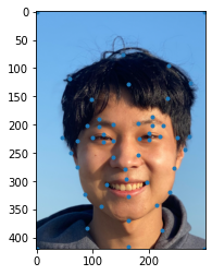
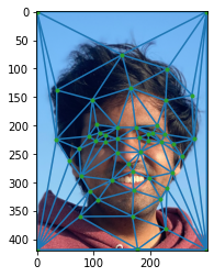
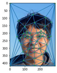
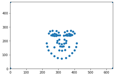
The starting point of everything is to define corresponding points between two faces. We do this using the ginput command from Python. We ensure that the labeling order is consistent between the two faces. You can see this labeling above. Note that we're looking for important features. Semantically, this intuitively lends to the corners/edges associated with the eyes, face shape, mouth, eyebrows, and nose.

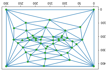
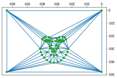
We can then average out each of the correspondences to generate the average shape of the two men. We then use this to create a triangular Delaunay mesh (using the built in scipy function). A visualization of the mesh is above.

The triangulation gives you what vertices make the best triangle. Since we picked the correspondences appropriately (in the same order), it is easy for us to be able to find what key points in each image make the best triangles given by the Delaunay mesh. This is visualized above in Figure 4.

Note that we only make ONE Delaunay mesh. We choose to do the middle one because it is the midpoint, so it is likely that both images can be bent to meet that mesh. Figure 4 is a representation of the triangles generated in the mean Delaunay mesh with the appropriate keypoints relevant to the image.

Part 2: Computing the Midway Face

Now that we have split the image into triangular meshes that correspond to each other, we can begin creating merged faces. One of the more meaningful of these is the halfway point: half-Amay and half-Alvin. To generate this image, we must perform two procedures.

The first is a warp: we are interested in getting the structure of the face. For the midway face, we have already done this. We've taken the mean of all the correspondences, since we needed this for the Delaunay triangulation.

The second procedure is a cross-dissolve. For each of the triangles in the midway face, we need half of the coloring to come from Amay and the other half from Alvin. We can fill this in reasonably easily. For each triangle in the midway face, we perform an inverse transformation. That is to say, for each pixel in the triangle, we find the transformation to the "pixel" coordinate that's in the corresponding triangle in Amay's face and the "pixel" coordinate that's in the corresponding triangle in Alvin's face. There's quite a bit to unpack here.

Firstly, why do we say "pixel" in quotes? In reality, the transformation back to Amay or Alvin's face may land us in between pixels. As such, we use an interpolation feature such as scipy's RectBivariateSpline to interpolate what color should correspond to that in-between place of pixels.

Secondly, how do we get this transformation? We know this transformation to be affine (translation, rotation, and scaling). As such, it can be represented as below.

Here, we are solving for 6 unknowns a-f. However, each triangle has 3 points, each with an x, y coordinate. This means that we have 6 knowns, so we can solve for these 6 unknowns by simply solving a system of linear equations. We can thus find the transform between (both directions, since we can take the inverse) each triangle in the desired midway image and the source images.

Now that we have this, we can get the color of each pixel in the midway image by averaging the color between the corresponding pixels of the triangles in Amay's and Alvin's faces. The results are shown below.

It's neat to see that this is different from simple alpha-blending. The features are aligned, so there are no duplicate features--no duplicate noses, no duplicate mouths, etc. This means the geometric warp to the average was successful. The lack of visual artifacts suggests the appearance cross-dissolve was successful as well.

Also, for the record, Amalvin has the kindest face and cutest cheeks ever. This photo made me super happy.

Part 3: The Morph Sequence

It is fairly intuitive to extrapolate out what we did to generate the midway face into making the morph sequence. Instead of taking the pure average, we take the weighted average. We can create 45 alphas evenly-spaced between [0, 1]. Each of the 45 alphas corresponds to a frame This alpha dictates how much of each component image weighs in on the frame. Amay gets an (1 - alpha) factor, and Alvin gets an (alpha) factor. This alpha factor applies to both the geometry and the cross-dissolve. This means that Amay's geometry (dictated by correspondence points) and coloring are stronger in the earlier frames, and Alvin's geometry and coloring are stronger in later frames. This creates a smooth transition. See the result below.

The geometry is fairly easy to notice moving from Amay to Alvin. You can tell the cross-dissolve alpha is at play too; Amay's skin tone is a little darker than Alvin's, and this checks out with the way the morph gif plays out. Note again that there are no duplicates of features--they merely grow/shrink according to the target.

Part 4: The "Mean Face" of a Population

Part 4.1: The average face shape

For this part, I used this dataset of faces of Danish computer scienists. This dataset comes pre-aligned and pre-annotated with correspondences of keypoints. As such, it was pretty straightforward to generate the mean face. To spice things up, I only took the color images of smiling men, so I created the mean male Danish computer scientist face in color, as shown in Figure 8 above.

To do generate the mean, I first created the mean geometric structure by averaging (weighting equally) each correspondence instance (Figure 8A). I then created the Delaunay mesh from this (Figure 8B). I could then use the correspondences and Delaunay mesh to warp the faces to mean and then average all pixels to create the average image.

Part 4.2: Morph each face to the average shape

Once you have the mean shape, you can warp the faces to match this geometric shape. We do the same procedure as in Parts 2 and 3. We inverse map each pixel from the triangles in the altered face to get some color from the source image. We do not do the cross-dissolve though; we keep the original coloring. This gives us the purely geometric warp to the mean. Some faces look a bit more natural than others. See Figure 9 for some samples.

As you can see above, some of these warps turn out better than others. Some factors include how well the person is aligned with others/the average as well as how unique the person's facial structure is. Figure 9A's warm to 9B looks reasonable--which is to say 9B looks like it could be a real person. Figure 9C to 9D's transformation is a little less natural; it looks as though the photo were taken at a bad angle or the subject had just been stung by wasps. This is likely because of the person's facial structure deviating from the norm. In Figure 9E to 9F, there's a much more pronounced error, largely because of the angle the original photo (9E) was taken at. It was not taken straight on, so the warping is a little unflattering. And not to be rude, but in some cases like FIgure 9G to 9H, the warp makes the person look a little more normal.

Part 4.3: Find the average face

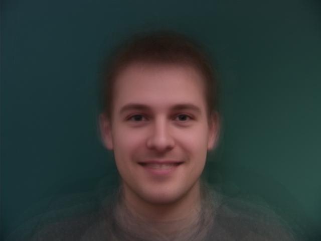
All this said and done, once all the faces have been warped to the mean, you can take the average of all the images (without having to do any additional Delaunay triangulaziation) across all pixels, since the images should line up nicely now. The result is shown below in Figure 10.

Note that the face is distinct, but the edges are a little fuzzy. This is because the correspondences were chosen with respect to mouth, nose, eyes, and chin. These features are reasonably well defined in this average, but others are fuzzy since we did not care to match for them.

Part 4.4: Me vs The Mean

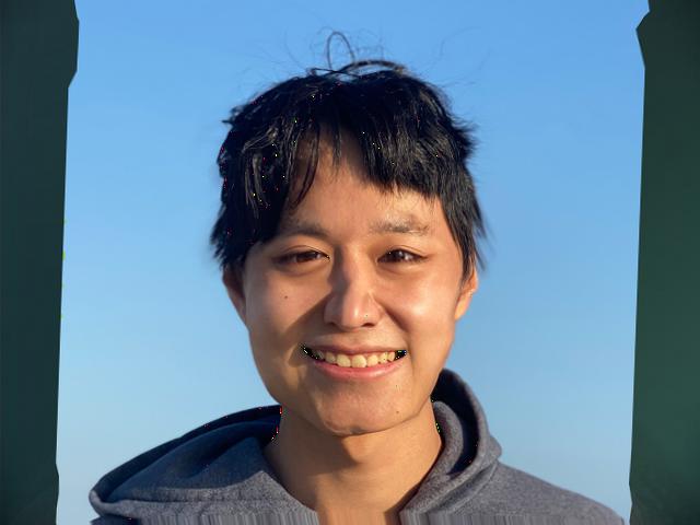
The subheading is misleading; in this portion, I'll be using Alvin's face again to see how he relates to the mean. This time, his face is aligned to the Dane's, and the contrasting background is due to the fact the Alvin photo is portrait mode instead of horizontal, so I pad the edges with the Danes' background.

Using the same techniques as 4.3, we can warp his face to the average Dane. The only difference is that I collected new correspondences between the generated average image and Alvin's face for the Delaunay triangularization. I used these same correspondences to warp the average Dane's face into Alvin's geometry.

As you can see, the results are pretty wonky. In Figure 11A, you can see that Alvin's eyes are shifted donwards as opposed to his usual up. His nose is elongated, and his jaw pushed in. All of this is more in line with what you expect of European (especially Danish) features. On the other hand, in Figure 11B, you can see some of the more distinct characteristics of Alvin: his left eyebrow quirks up and his left cheek sticks out a little more (based on the angle of the photo).

Part 5: Caricatures: Extrapolating from the Mean

Because faces constitute a subspace, we can do wonky things with them. We can subtract two and call the difference vector a meaningful direction. As such, if instead of taking the average (as we did in Part 2) or even taking weighted averages between images (as we did in Part 3), we can instead EXTRAPOLATE instead of interpolate. This extrapolation is intuitively meaningful. If we weight the Danish correspondence points by a -X amount and the Alvin correspondence points by a +Y amount (such that -X + Y = 1) , we can generate a face that amplifies the features that are unique to Alvin. This is, in short, a caricature. We see the results below.

As you can see, as the magnitude of -X and Y each get bigger, the features that make Alvin unique get bigger. In Figure 12A we notice the left cheek bulge is a little bigger. In Figure 12B, the left eyebrow is substantially quirked up. In Figure 12C, we start to notice the hair get pulled out on the left too (since he has such a charmingly terrible haircut). In Figure 12D, with such a far-out extrapolation, the naturalness of his facial features deteriorates a lot more, and his eyes are substantially smaller (especially with respect to a Dane's). These caricatures do emphasize the features that distinguish Alvin from the Danes.

Part 6: Bells & Whistles: Exploring Gender

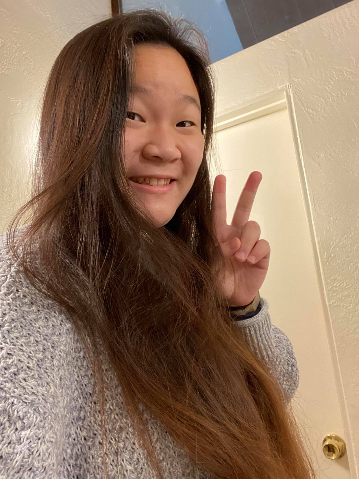
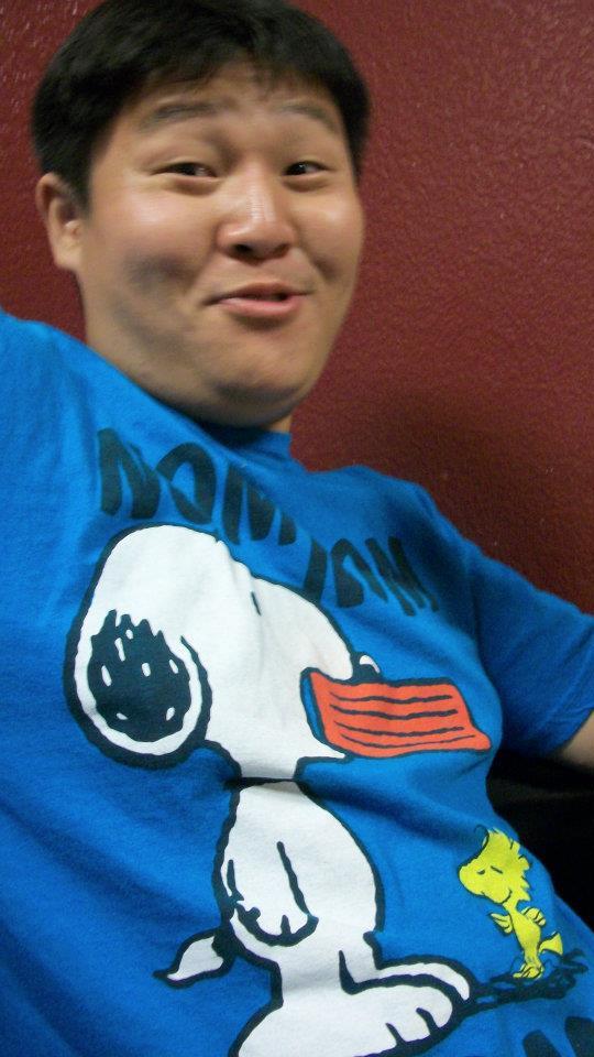
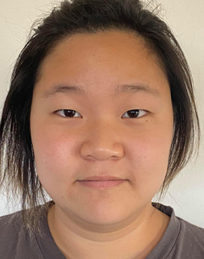
For the open-ended part of this project, I wanted to explore shifting the gender of my face towards the male end of the spectrum. This was mainly out of curiosity to see if I'd look more like my brother. Reference photos above.

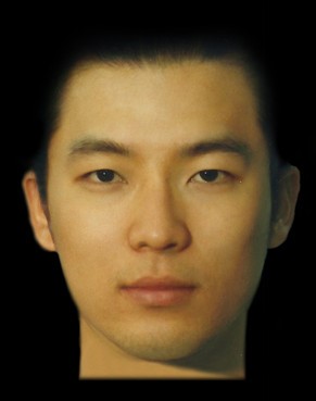
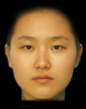
To do this, I found an article with a Korean research institute's results for average Korean male and female faces. These are shown in Figure 14.

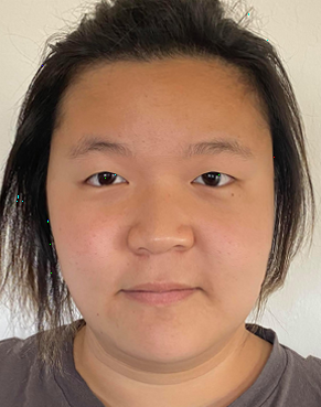
It's important that these faces be Korean so they are the most similar to my brother's and my own. We are most interested in exploring gender, not any other factors. Using the averages for the Korean populaton helps us constrain the experiment so we are looking only at the variable of interest. For us, we are only interested in looking at the average Korean male face. As such, I collected correspondences between Figure 14A and a picture of myself that is well aligned (Figure 15A).

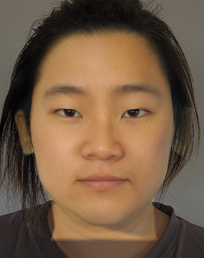
I did a shape morph, color morph, and full morph. The shape morph (Figure 15B) is done by taking the Delaunay triangularization from the correspondences in the average Korean male face. I then populated the triangles with colors exclusively from my face. As you can see, this is a little bit wonky. It makes the angles in my face more sharp, and my face appears to be overall longer. My eyes look like the corners have been tilted down.

To do the color morph (Figure 15C), I did what was suggested by Kamyar on Piazza: the mean face was warped to my geometry and cross dissolved. I did not use exclusively colors from the average Korean male face since I wanted the resulting image to still look like me. This photo looks much less like me, even with some of the colors from my photo. The eyes, however, are tilted up like mine are. The nose does look tilted though.

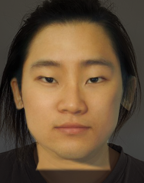
To get the full effect, I did a full morph as well (Figure 15D). For this, my face was mapped to the average Korean male face. The coloring was done with an equal weighting between my face and the average Korean male face. This photo has a component that is more obviously me than 15C. However, it does look substantially more masculine, thanks to the sharper edges and longer face.

All that being said and done, male me does not look more like my brother than regular old me. This is a little bit disappointing, given that people are always telling us how much we look alike.

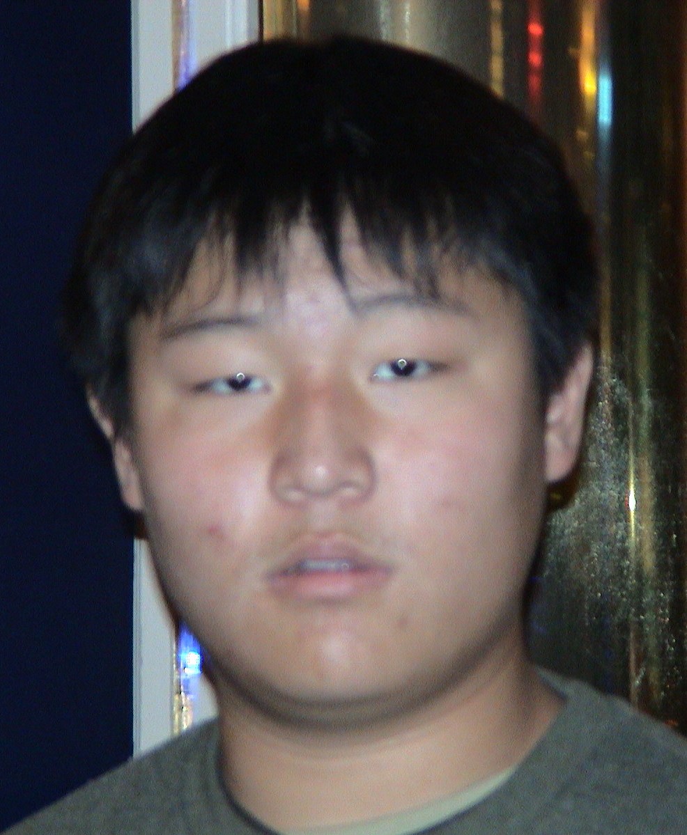
More Bells & Whistles: Family Matters

To try to attempt to get closer to my brother, I did a combination of morphs with my father.

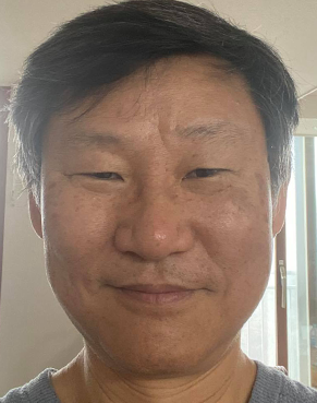
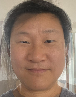
This is the most promising result I got. Using my father's geometry with a 35-65 Stella-Dad split, I get a picture that looks kind of like my brother if you squint. And my brother got very old. I guess I will show this to him and let him know that this is what he has to look forward to in 15 years.